# Import required libraries
import numpy as np
import pandas as pd
import matplotlib.pyplot as plt
from sklearn.model_selection import train_test_split
from sklearn.preprocessing import StandardScaler
from sklearn.metrics import mean_squared_error, r2_score, mean_absolute_error
from sklearn.linear_model import LinearRegression, Ridge, Lasso
from sklearn.svm import SVR
import warnings
warnings.filterwarnings('ignore')18 scikit-learn: Regression
18.1 Introduction to Regression
Regression is a supervised learning technique used to predict continuous numerical values. Unlike classification which predicts discrete categories, regression models predict quantities such as prices, temperatures, sales figures, or any other continuous variable.
In this tutorial, we’ll explore four fundamental regression algorithms from scikit-learn:
- Linear Regression: The foundation of regression analysis
- Ridge Regression: Linear regression with L2 regularization
- Lasso Regression: Linear regression with L1 regularization
- Support Vector Regression (SVR): Non-linear regression using support vector machines
18.2 Prerequisites
Before we begin, make sure you have the required packages installed:
18.3 Sample Dataset
Let’s create a sample dataset for demonstration purposes:
# Set random seed for reproducibility
np.random.seed(42)

# Generate sample data
n_samples = 200
X = np.random.randn(n_samples, 5)
# Create target variable with some noise
y = 3*X[:, 0] + 2*X[:, 1] - 1.5*X[:, 2] + 0.5*X[:, 3] + np.random.randn(n_samples) * 0.5

# Split the data
X_train, X_test, y_train, y_test = train_test_split(X, y, test_size=0.2, random_state=42)

print(f"Training set size: {X_train.shape}")
print(f"Test set size: {X_test.shape}")
Training set size: (160, 5)
Test set size: (40, 5)18.4 Linear Regression
18.5 Overview
Linear Regression is the most basic and widely used regression algorithm. It assumes a linear relationship between the input features and the target variable.
Mathematical Formula:
\[ y = \beta_0 + \beta_1 x_1 + \beta_2 x_2 + ... + \beta_n x_n \]
Where: - \(y\) is the predicted value - \(\beta_0\) is the intercept - \(\beta_1, \beta_2, ..., \beta_n\) are coefficients - \(x_1, x_2, ..., x_n\) are features
18.6 Key Characteristics
- Pros: Simple, interpretable, fast to train
- Cons: Assumes linear relationship, sensitive to outliers, prone to overfitting with many features
- Use Cases: When relationships are approximately linear, baseline model for comparison
18.7 Implementation
# Create and train Linear Regression model
lr_model = LinearRegression()
lr_model.fit(X_train, y_train)

# Make predictions
y_pred_lr = lr_model.predict(X_test)

# Evaluate the model
lr_mse = mean_squared_error(y_test, y_pred_lr)
lr_rmse = np.sqrt(lr_mse)
lr_r2 = r2_score(y_test, y_pred_lr)
lr_mae = mean_absolute_error(y_test, y_pred_lr)

print("Linear Regression Performance:")
print(f"Mean Squared Error (MSE): {lr_mse:.4f}")
print(f"Root Mean Squared Error (RMSE): {lr_rmse:.4f}")
print(f"R² Score: {lr_r2:.4f}")
print(f"Mean Absolute Error (MAE): {lr_mae:.4f}")
print(f"\nCoefficients: {lr_model.coef_}")
print(f"Intercept: {lr_model.intercept_:.4f}")
Linear Regression Performance:
Mean Squared Error (MSE): 0.2295
Root Mean Squared Error (RMSE): 0.4790
R² Score: 0.9857
Mean Absolute Error (MAE): 0.4111
Coefficients: [ 2.97001147 2.02962236 -1.50521429 0.51827429 0.02157209]
Intercept: 0.068518.8 Visualization
# Plot predictions vs actual values
plt.figure(figsize=(10, 6))
plt.scatter(y_test, y_pred_lr, alpha=0.6, edgecolors='k')
plt.plot([y_test.min(), y_test.max()], [y_test.min(), y_test.max()], 'r--', lw=2, label='Perfect Prediction')
plt.xlabel('Actual Values')
plt.ylabel('Predicted Values')
plt.title('Linear Regression: Predicted vs Actual')
plt.legend()
plt.grid(True, alpha=0.3)
plt.tight_layout()
plt.show()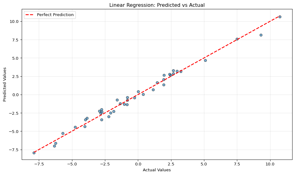
18.9 Ridge Regression
18.10 Overview
Ridge Regression (also known as L2 regularization) adds a penalty term to the linear regression cost function to prevent overfitting. It’s particularly useful when dealing with multicollinearity or when you have many features.
Mathematical Formula:
\[ \text{Cost} = \sum_{i=1}^{n} (y_i - \hat{y}_i)^2 + \alpha \sum_{j=1}^{p} \beta_j^2 \]
Where: - \(\alpha\) is the regularization parameter - The second term is the L2 penalty (sum of squared coefficients)
18.11 Key Characteristics
- Pros: Handles multicollinearity well, reduces overfitting, keeps all features
- Cons: Doesn’t perform feature selection, requires tuning of alpha parameter
- Use Cases: When you have correlated features, many features relative to samples
18.12 Implementation
# Create and train Ridge Regression model
ridge_model = Ridge(alpha=1.0)  # alpha is the regularization strength
ridge_model.fit(X_train, y_train)

# Make predictions
y_pred_ridge = ridge_model.predict(X_test)

# Evaluate the model
ridge_mse = mean_squared_error(y_test, y_pred_ridge)
ridge_rmse = np.sqrt(ridge_mse)
ridge_r2 = r2_score(y_test, y_pred_ridge)
ridge_mae = mean_absolute_error(y_test, y_pred_ridge)

print("Ridge Regression Performance:")
print(f"Mean Squared Error (MSE): {ridge_mse:.4f}")
print(f"Root Mean Squared Error (RMSE): {ridge_rmse:.4f}")
print(f"R² Score: {ridge_r2:.4f}")
print(f"Mean Absolute Error (MAE): {ridge_mae:.4f}")
print(f"\nCoefficients: {ridge_model.coef_}")
print(f"Intercept: {ridge_model.intercept_:.4f}")
Ridge Regression Performance:
Mean Squared Error (MSE): 0.2311
Root Mean Squared Error (RMSE): 0.4807
R² Score: 0.9856
Mean Absolute Error (MAE): 0.4097
Coefficients: [ 2.94483134 2.0144098 -1.4906361 0.51389808 0.0195997 ]
Intercept: 0.069018.13 Hyperparameter Tuning
# Test different alpha values
alphas = [0.001, 0.01, 0.1, 1.0, 10.0, 100.0]
ridge_scores = []

for alpha in alphas:
    ridge = Ridge(alpha=alpha)
    ridge.fit(X_train, y_train)
    score = ridge.score(X_test, y_test)
    ridge_scores.append(score)
    print(f"Alpha: {alpha:6.3f} | R² Score: {score:.4f}")

# Plot alpha vs R² score
plt.figure(figsize=(10, 6))
plt.plot(alphas, ridge_scores, marker='o', linewidth=2, markersize=8)
plt.xscale('log')
plt.xlabel('Alpha (Regularization Strength)')
plt.ylabel('R² Score')
plt.title('Ridge Regression: Alpha vs Model Performance')
plt.grid(True, alpha=0.3)
plt.tight_layout()
plt.show()
Alpha: 0.001 | R² Score: 0.9857
Alpha: 0.010 | R² Score: 0.9857
Alpha: 0.100 | R² Score: 0.9857
Alpha: 1.000 | R² Score: 0.9856
Alpha: 10.000 | R² Score: 0.9793
Alpha: 100.000 | R² Score: 0.7742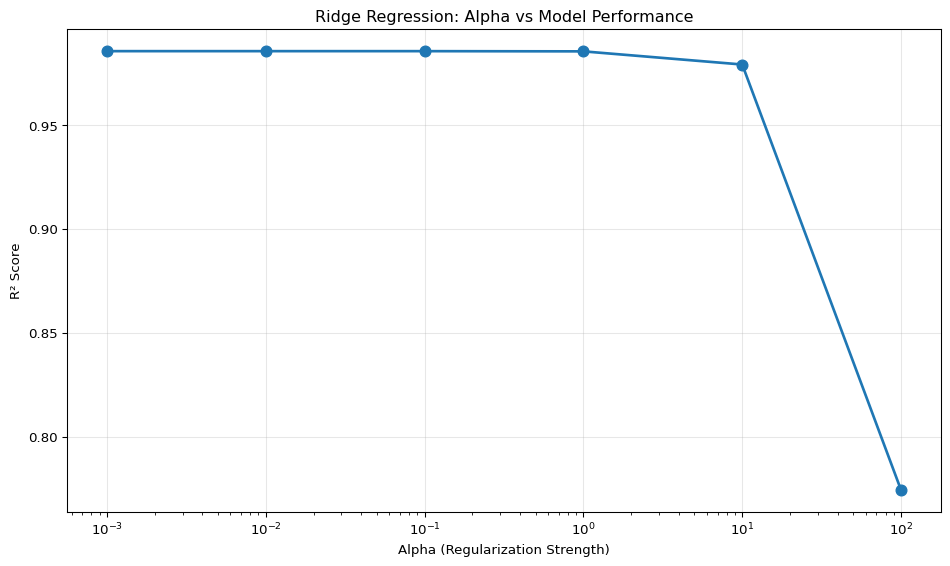
18.14 Lasso Regression
18.15 Overview
Lasso Regression (Least Absolute Shrinkage and Selection Operator) uses L1 regularization, which can shrink some coefficients to exactly zero, effectively performing feature selection.
Mathematical Formula:
\[ \text{Cost} = \sum_{i=1}^{n} (y_i - \hat{y}_i)^2 + \alpha \sum_{j=1}^{p} |\beta_j| \]
Where: - \(\alpha\) is the regularization parameter - The second term is the L1 penalty (sum of absolute coefficients)
18.16 Key Characteristics
- Pros: Performs automatic feature selection, creates sparse models, handles multicollinearity
- Cons: May arbitrarily select one feature among correlated features, requires tuning of alpha
- Use Cases: When you suspect only a subset of features are important, high-dimensional data
18.17 Implementation
# Create and train Lasso Regression model
lasso_model = Lasso(alpha=0.1)  # alpha is the regularization strength
lasso_model.fit(X_train, y_train)

# Make predictions
y_pred_lasso = lasso_model.predict(X_test)

# Evaluate the model
lasso_mse = mean_squared_error(y_test, y_pred_lasso)
lasso_rmse = np.sqrt(lasso_mse)
lasso_r2 = r2_score(y_test, y_pred_lasso)
lasso_mae = mean_absolute_error(y_test, y_pred_lasso)

print("Lasso Regression Performance:")
print(f"Mean Squared Error (MSE): {lasso_mse:.4f}")
print(f"Root Mean Squared Error (RMSE): {lasso_rmse:.4f}")
print(f"R² Score: {lasso_r2:.4f}")
print(f"Mean Absolute Error (MAE): {lasso_mae:.4f}")
print(f"\nCoefficients: {lasso_model.coef_}")
print(f"Intercept: {lasso_model.intercept_:.4f}")
print(f"\nNumber of non-zero coefficients: {np.sum(lasso_model.coef_ != 0)}")
Lasso Regression Performance:
Mean Squared Error (MSE): 0.3073
Root Mean Squared Error (RMSE): 0.5544
R² Score: 0.9809
Mean Absolute Error (MAE): 0.4580
Coefficients: [ 2.81877725 1.91572643 -1.36280794 0.39858682 -0. ]
Intercept: 0.0759
Number of non-zero coefficients: 418.18 Feature Selection Visualization
# Visualize feature importance (coefficients)
feature_names = [f'Feature {i+1}' for i in range(X.shape[1])]

plt.figure(figsize=(10, 6))
plt.bar(feature_names, lasso_model.coef_, alpha=0.7, edgecolor='black')
plt.axhline(y=0, color='r', linestyle='--', linewidth=1)
plt.xlabel('Features')
plt.ylabel('Coefficient Value')
plt.title('Lasso Regression: Feature Coefficients (Feature Selection)')
plt.grid(True, alpha=0.3, axis='y')
plt.tight_layout()
plt.show()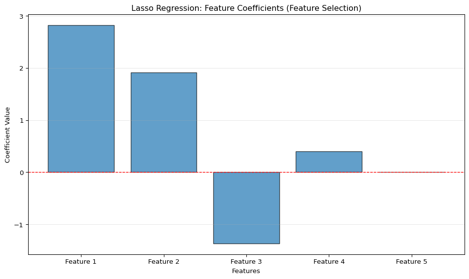
18.19 Comparing Different Alpha Values
# Test different alpha values for Lasso
alphas_lasso = [0.001, 0.01, 0.1, 1.0, 10.0]
lasso_scores = []
non_zero_coefs = []

for alpha in alphas_lasso:
    lasso = Lasso(alpha=alpha)
    lasso.fit(X_train, y_train)
    score = lasso.score(X_test, y_test)
    lasso_scores.append(score)
    non_zero_coefs.append(np.sum(lasso.coef_ != 0))
    print(f"Alpha: {alpha:6.3f} | R² Score: {score:.4f} | Non-zero features: {non_zero_coefs[-1]}")
Alpha: 0.001 | R² Score: 0.9857 | Non-zero features: 5
Alpha: 0.010 | R² Score: 0.9857 | Non-zero features: 5
Alpha: 0.100 | R² Score: 0.9809 | Non-zero features: 4
Alpha: 1.000 | R² Score: 0.6112 | Non-zero features: 3
Alpha: 10.000 | R² Score: -0.0097 | Non-zero features: 018.20 Support Vector Regression (SVR)
18.21 Overview
Support Vector Regression (SVR) is based on Support Vector Machine (SVM) principles. Unlike linear models, SVR can capture non-linear relationships using kernel functions. It tries to fit the best line within a threshold epsilon (ε).
Key Concepts:
- Uses kernel trick to handle non-linear relationships
- Focuses on data points within epsilon margin
- Less sensitive to outliers outside the margin
18.22 Key Characteristics
- Pros: Handles non-linear relationships, robust to outliers, effective in high dimensions
- Cons: Slower training on large datasets, requires feature scaling, multiple hyperparameters to tune
- Use Cases: Non-linear relationships, when you need robustness to outliers
18.23 Implementation with Linear Kernel
# Feature scaling (important for SVR!)
scaler = StandardScaler()
X_train_scaled = scaler.fit_transform(X_train)
X_test_scaled = scaler.transform(X_test)

# Create and train SVR model with linear kernel
svr_linear = SVR(kernel='linear', C=1.0)
svr_linear.fit(X_train_scaled, y_train)

# Make predictions
y_pred_svr_linear = svr_linear.predict(X_test_scaled)

# Evaluate the model
svr_linear_mse = mean_squared_error(y_test, y_pred_svr_linear)
svr_linear_rmse = np.sqrt(svr_linear_mse)
svr_linear_r2 = r2_score(y_test, y_pred_svr_linear)
svr_linear_mae = mean_absolute_error(y_test, y_pred_svr_linear)

print("SVR (Linear Kernel) Performance:")
print(f"Mean Squared Error (MSE): {svr_linear_mse:.4f}")
print(f"Root Mean Squared Error (RMSE): {svr_linear_rmse:.4f}")
print(f"R² Score: {svr_linear_r2:.4f}")
print(f"Mean Absolute Error (MAE): {svr_linear_mae:.4f}")
SVR (Linear Kernel) Performance:
Mean Squared Error (MSE): 0.2432
Root Mean Squared Error (RMSE): 0.4932
R² Score: 0.9849
Mean Absolute Error (MAE): 0.423018.24 Implementation with RBF Kernel
# Create and train SVR model with RBF (Radial Basis Function) kernel
svr_rbf = SVR(kernel='rbf', C=1.0, gamma='scale')
svr_rbf.fit(X_train_scaled, y_train)

# Make predictions
y_pred_svr_rbf = svr_rbf.predict(X_test_scaled)

# Evaluate the model
svr_rbf_mse = mean_squared_error(y_test, y_pred_svr_rbf)
svr_rbf_rmse = np.sqrt(svr_rbf_mse)
svr_rbf_r2 = r2_score(y_test, y_pred_svr_rbf)
svr_rbf_mae = mean_absolute_error(y_test, y_pred_svr_rbf)

print("SVR (RBF Kernel) Performance:")
print(f"Mean Squared Error (MSE): {svr_rbf_mse:.4f}")
print(f"Root Mean Squared Error (RMSE): {svr_rbf_rmse:.4f}")
print(f"R² Score: {svr_rbf_r2:.4f}")
print(f"Mean Absolute Error (MAE): {svr_rbf_mae:.4f}")
SVR (RBF Kernel) Performance:
Mean Squared Error (MSE): 3.4360
Root Mean Squared Error (RMSE): 1.8536
R² Score: 0.7865
Mean Absolute Error (MAE): 1.219818.25 Kernel Comparison
# Compare different kernels
kernels = ['linear', 'rbf', 'poly']
svr_results = {}

for kernel in kernels:
    svr = SVR(kernel=kernel, C=1.0)
    svr.fit(X_train_scaled, y_train)
    y_pred = svr.predict(X_test_scaled)
    r2 = r2_score(y_test, y_pred)
    rmse = np.sqrt(mean_squared_error(y_test, y_pred))
    svr_results[kernel] = {'R²': r2, 'RMSE': rmse}
    print(f"{kernel.upper()} Kernel - R²: {r2:.4f}, RMSE: {rmse:.4f}")
LINEAR Kernel - R²: 0.9849, RMSE: 0.4932
RBF Kernel - R²: 0.7865, RMSE: 1.8536
POLY Kernel - R²: 0.7974, RMSE: 1.805418.26 Model Comparison
18.27 Performance Summary
Let’s compare all four regression models:
# Create comparison dataframe
comparison_df = pd.DataFrame({
    'Model': ['Linear Regression', 'Ridge Regression', 'Lasso Regression', 'SVR (RBF)'],
    'MSE': [lr_mse, ridge_mse, lasso_mse, svr_rbf_mse],
    'RMSE': [lr_rmse, ridge_rmse, lasso_rmse, svr_rbf_rmse],
    'R² Score': [lr_r2, ridge_r2, lasso_r2, svr_rbf_r2],
    'MAE': [lr_mae, ridge_mae, lasso_mae, svr_rbf_mae]
})

print("Model Performance Comparison:")
print(comparison_df.to_string(index=False))
Model Performance Comparison:
Model MSE RMSE R² Score MAE
Linear Regression 0.229482 0.479043 0.985738 0.411104
Ridge Regression 0.231105 0.480734 0.985637 0.409747
Lasso Regression 0.307348 0.554389 0.980899 0.457962
SVR (RBF) 3.435965 1.853635 0.786457 1.21977718.28 Visual Comparison
# Create visualization comparing all models
fig, axes = plt.subplots(2, 2, figsize=(14, 10))

models = [
    ('Linear Regression', y_pred_lr),
    ('Ridge Regression', y_pred_ridge),
    ('Lasso Regression', y_pred_lasso),
    ('SVR (RBF)', y_pred_svr_rbf)
]

for idx, (name, predictions) in enumerate(models):
    ax = axes[idx // 2, idx % 2]
    ax.scatter(y_test, predictions, alpha=0.6, edgecolors='k')
    ax.plot([y_test.min(), y_test.max()], [y_test.min(), y_test.max()],
            'r--', lw=2, label='Perfect Prediction')
    ax.set_xlabel('Actual Values')
    ax.set_ylabel('Predicted Values')
    ax.set_title(f'{name}')
    ax.legend()
    ax.grid(True, alpha=0.3)

plt.tight_layout()
plt.show()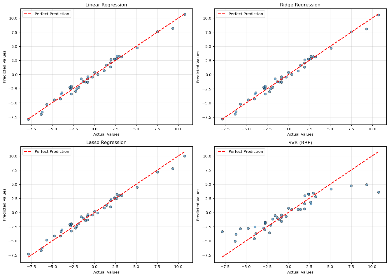
18.29 Bar Chart Comparison
# Create bar chart for R² scores
fig, (ax1, ax2) = plt.subplots(1, 2, figsize=(14, 5))

# R² Score comparison
models_names = comparison_df['Model']
r2_scores = comparison_df['R² Score']

ax1.bar(models_names, r2_scores, alpha=0.7, edgecolor='black', color=['#1f77b4', '#ff7f0e', '#2ca02c', '#d62728'])
ax1.set_ylabel('R² Score')
ax1.set_title('Model Comparison: R² Score (Higher is Better)')
ax1.set_ylim([0, 1])
ax1.grid(True, alpha=0.3, axis='y')
ax1.tick_params(axis='x', rotation=45)

# RMSE comparison
rmse_scores = comparison_df['RMSE']

ax2.bar(models_names, rmse_scores, alpha=0.7, edgecolor='black', color=['#1f77b4', '#ff7f0e', '#2ca02c', '#d62728'])
ax2.set_ylabel('RMSE')
ax2.set_title('Model Comparison: RMSE (Lower is Better)')
ax2.grid(True, alpha=0.3, axis='y')
ax2.tick_params(axis='x', rotation=45)

plt.tight_layout()
plt.show()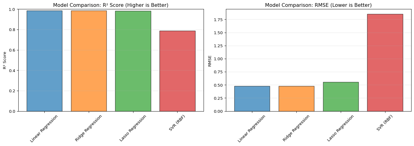
19 Choosing the Right Model
19.1 Decision Guide
| Model | When to Use | When to Avoid |
|---|---|---|
| Linear Regression | - Simple baseline model - Linear relationships - Interpretability is key - Small to medium datasets |
- Non-linear relationships - Many correlated features - High-dimensional data |
| Ridge Regression | - Multicollinearity present - Many features - Want to keep all features - Prevent overfitting |
- Need feature selection - Truly sparse models required |
| Lasso Regression | - Feature selection needed - Sparse models desired - High-dimensional data - Believe few features matter |
- Need all features - Uncertain about feature importance |
| SVR | - Non-linear relationships - Robust to outliers needed - Complex patterns - High-dimensional space |
- Very large datasets (slow) - Real-time predictions needed - Interpretability critical |
19.2 Key Hyperparameters
Ridge and Lasso
- alpha: Regularization strength
- Higher values = more regularization = simpler models
- Use cross-validation to find optimal value
SVR
- kernel: Type of kernel function (‘linear’, ‘rbf’, ‘poly’, ‘sigmoid’)
- C: Regularization parameter (inverse of alpha)
- Lower values = more regularization
- gamma: Kernel coefficient (for ‘rbf’, ‘poly’, ‘sigmoid’)
- Higher values = more complex decision boundary
- epsilon: Size of epsilon-tube (no penalty for errors within this range)
19.3 Best Practices
19.4 Data Preprocessing
# Always split data before preprocessing
X_train, X_test, y_train, y_test = train_test_split(X, y, test_size=0.2, random_state=42)

# Scale features (especially important for SVR and regularized models)
scaler = StandardScaler()
X_train_scaled = scaler.fit_transform(X_train)  # Fit on training data only
X_test_scaled = scaler.transform(X_test)  # Transform test data
19.5 Model Evaluation
# Use multiple metrics
from sklearn.metrics import mean_squared_error, r2_score, mean_absolute_error

def evaluate_model(y_true, y_pred, model_name):
    """Comprehensive model evaluation"""
    mse = mean_squared_error(y_true, y_pred)
    rmse = np.sqrt(mse)
    mae = mean_absolute_error(y_true, y_pred)
    r2 = r2_score(y_true, y_pred)

    print(f"\n{model_name} Performance:")
    print(f"  RMSE: {rmse:.4f}")
    print(f"  MAE:  {mae:.4f}")
    print(f"  R²:   {r2:.4f}")

    return {'RMSE': rmse, 'MAE': mae, 'R²': r2}
19.6 Cross-Validation
from sklearn.model_selection import cross_val_score

# Perform k-fold cross-validation
def cross_validate_model(model, X, y, cv=5):
    """Perform cross-validation and return scores"""
    scores = cross_val_score(model, X, y, cv=cv, scoring='r2')
    print(f"Cross-validation R² scores: {scores}")
    print(f"Mean R²: {scores.mean():.4f} (+/- {scores.std() * 2:.4f})")
    return scores

# Example usage
lr = LinearRegression()
cross_validate_model(lr, X_train, y_train, cv=5)
Cross-validation R² scores: [0.96763478 0.96922656 0.96834017 0.98373304 0.97486871]
Mean R²: 0.9728 (+/- 0.0121)array([0.96763478, 0.96922656, 0.96834017, 0.98373304, 0.97486871])19.7 Hyperparameter Tuning
from sklearn.model_selection import GridSearchCV

# Example: Tuning Ridge Regression
param_grid = {
    'alpha': [0.001, 0.01, 0.1, 1.0, 10.0, 100.0]
}

ridge = Ridge()
grid_search = GridSearchCV(ridge, param_grid, cv=5, scoring='r2')
grid_search.fit(X_train, y_train)

print(f"Best parameters: {grid_search.best_params_}")
print(f"Best cross-validation score: {grid_search.best_score_:.4f}")

# Use best model
best_ridge = grid_search.best_estimator_
Best parameters: {'alpha': 0.1}
Best cross-validation score: 0.972820 Real-World Example: House Price Prediction
Let’s apply what we’ve learned to a practical example:
# Create a more realistic dataset simulating house prices
np.random.seed(42)
n_houses = 500

# Features: square footage, bedrooms, bathrooms, age, distance to city center
square_footage = np.random.normal(2000, 500, n_houses)
bedrooms = np.random.randint(1, 6, n_houses)
bathrooms = np.random.randint(1, 4, n_houses)
age = np.random.randint(0, 50, n_houses)
distance = np.random.uniform(0, 30, n_houses)

# Create feature matrix
X_houses = np.column_stack([square_footage, bedrooms, bathrooms, age, distance])

# Generate prices with realistic relationships
base_price = 100000
price = (base_price +
         150 * square_footage +
         25000 * bedrooms +
         15000 * bathrooms -
         800 * age -
         2000 * distance +
         np.random.normal(0, 20000, n_houses))

# Split the data
X_train_h, X_test_h, y_train_h, y_test_h = train_test_split(
    X_houses, price, test_size=0.2, random_state=42
)

# Scale features
scaler_h = StandardScaler()
X_train_h_scaled = scaler_h.fit_transform(X_train_h)
X_test_h_scaled = scaler_h.transform(X_test_h)

# Try different models
models_house = {
    'Linear Regression': LinearRegression(),
    'Ridge': Ridge(alpha=1.0),
    'Lasso': Lasso(alpha=100),
    'SVR': SVR(kernel='rbf', C=100)
}

print("House Price Prediction Results:\n")
feature_names_house = ['Square Footage', 'Bedrooms', 'Bathrooms', 'Age', 'Distance to City']

for name, model in models_house.items():
    if name == 'SVR':
        model.fit(X_train_h_scaled, y_train_h)
        y_pred_h = model.predict(X_test_h_scaled)
    else:
        model.fit(X_train_h, y_train_h)
        y_pred_h = model.predict(X_test_h)

    r2 = r2_score(y_test_h, y_pred_h)
    rmse = np.sqrt(mean_squared_error(y_test_h, y_pred_h))

    print(f"{name}:")
    print(f"  R² Score: {r2:.4f}")
    print(f"  RMSE: ${rmse:,.2f}\n")
House Price Prediction Results:
Linear Regression:
R² Score: 0.9369
RMSE: $20,887.29
Ridge:
R² Score: 0.9369
RMSE: $20,892.09
Lasso:
R² Score: 0.9368
RMSE: $20,904.60
SVR:
R² Score: 0.0356
RMSE: $81,674.60
20.1 Conclusion
20.2 Summary
We’ve explored four fundamental regression algorithms in scikit-learn:
- Linear Regression: Fast, interpretable baseline model
- Ridge Regression: Handles multicollinearity with L2 regularization
- Lasso Regression: Performs feature selection with L1 regularization
- Support Vector Regression: Captures non-linear relationships
20.3 Key Takeaways
- Start with Linear Regression as a baseline
- Use Ridge when you have correlated features
- Use Lasso when you need automatic feature selection
- Use SVR for complex non-linear patterns
- Always scale your features, especially for SVR and regularized models
- Use cross-validation for reliable performance estimates
- Consider multiple evaluation metrics (R², RMSE, MAE)
20.4 Next Steps
To deepen your understanding:
- Experiment with real-world datasets (housing, stocks, weather)
- Practice hyperparameter tuning with GridSearchCV or RandomizedSearchCV
- Explore ensemble methods (Random Forest, Gradient Boosting)
- Learn about polynomial features for non-linear relationships
- Study advanced regularization techniques (ElasticNet)
20.5 Resources
Happy Modeling! 🚀