import numpy as np
import pandas as pd
import matplotlib.pyplot as plt
import seaborn as sns
from sklearn.model_selection import train_test_split
from sklearn.preprocessing import StandardScaler
from sklearn.metrics import accuracy_score, classification_report, confusion_matrix

# Set random seed for reproducibility
np.random.seed(42)

# Display settings
sns.set_style("whitegrid")
plt.rcParams['figure.figsize'] = (10, 6)16 scikit-learn: Classification
16.1 Introduction to Classification
Classification is a supervised machine learning task where we predict a category or class for new data based on patterns learned from labeled training data.
Real-world examples: - Email filtering: “spam” or “not spam” - Medical diagnosis: “disease” or “no disease” - Image recognition: “cat”, “dog”, or “bird” - Customer churn: “will leave” or “will stay”
In this tutorial, we’ll explore four popular classification algorithms from scikit-learn:
- Logistic Regression - Linear model for binary/multi-class classification
- k-Nearest Neighbors (KNN) - Instance-based learning
- Support Vector Machines (SVM) - Maximum margin classifier
- Decision Trees - Tree-based rule learning
16.2 Setup and Data Preparation
First, let’s import the necessary libraries and load a dataset:
Load the Iris Dataset
We’ll use the famous Iris dataset - a classic dataset for classification:
from sklearn.datasets import load_iris

# Load the dataset
iris = load_iris()
X = iris.data  # Features: sepal length, sepal width, petal length, petal width
y = iris.target  # Target: 0=setosa, 1=versicolor, 2=virginica

# Create a DataFrame for better visualization
df = pd.DataFrame(X, columns=iris.feature_names)
df['species'] = pd.Categorical.from_codes(y, iris.target_names)

print("Dataset shape:", X.shape)
print("\nFirst 5 rows:")
print(df.head())
print("\nClass distribution:")
print(df['species'].value_counts())
Dataset shape: (150, 4)
First 5 rows:
sepal length (cm) sepal width (cm) petal length (cm) petal width (cm) \
0 5.1 3.5 1.4 0.2
1 4.9 3.0 1.4 0.2
2 4.7 3.2 1.3 0.2
3 4.6 3.1 1.5 0.2
4 5.0 3.6 1.4 0.2
species
0 setosa
1 setosa
2 setosa
3 setosa
4 setosa
Class distribution:
species
setosa 50
versicolor 50
virginica 50
Name: count, dtype: int64Visualize the Data
# Create a pair plot to visualize relationships
plt.figure(figsize=(12, 10))
sns.pairplot(df, hue='species', markers=['o', 's', 'D'])
plt.suptitle('Iris Dataset: Feature Relationships', y=1.02)
plt.show()
<Figure size 1152x960 with 0 Axes>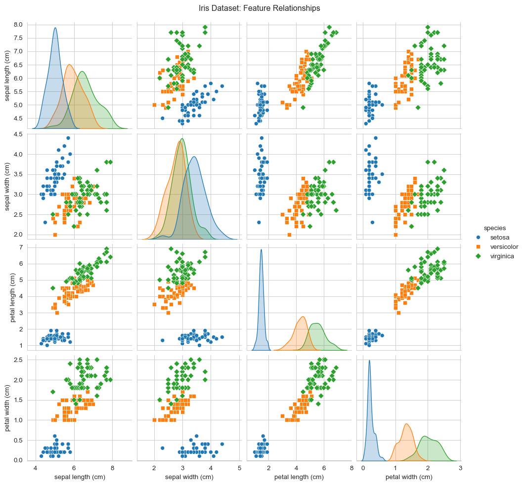
Split Data into Training and Test Sets
# Split the data: 80% training, 20% testing
X_train, X_test, y_train, y_test = train_test_split(
    X, y, test_size=0.2, random_state=42, stratify=y
)

print(f"Training set size: {X_train.shape[0]} samples")
print(f"Test set size: {X_test.shape[0]} samples")
print(f"\nTraining set class distribution: {np.bincount(y_train)}")
print(f"Test set class distribution: {np.bincount(y_test)}")
Training set size: 120 samples
Test set size: 30 samples
Training set class distribution: [40 40 40]
Test set class distribution: [10 10 10]Feature Scaling
Many algorithms perform better with scaled features:
# Standardize features (mean=0, std=1)
scaler = StandardScaler()
X_train_scaled = scaler.fit_transform(X_train)
X_test_scaled = scaler.transform(X_test)

print("Original feature ranges:")
print(pd.DataFrame(X_train, columns=iris.feature_names).describe().loc[['min', 'max']])
print("\nScaled feature ranges:")
print(pd.DataFrame(X_train_scaled, columns=iris.feature_names).describe().loc[['min', 'max']])
Original feature ranges:
sepal length (cm) sepal width (cm) petal length (cm) petal width (cm)
min 4.3 2.0 1.1 0.1
max 7.9 4.4 6.9 2.5
Scaled feature ranges:
sepal length (cm) sepal width (cm) petal length (cm) petal width (cm)
min -1.840983 -2.347097 -1.516067 -1.454945
max 2.457961 3.026225 1.777262 1.70511616.3 Logistic Regression
What it is: Despite its name, Logistic Regression is a classification algorithm that models the probability of a sample belonging to a particular class using a logistic (sigmoid) function.
How it works: - Uses a linear combination of features - Applies sigmoid function to get probabilities (0 to 1) - Best for linearly separable data
When to use: - ✅ Fast training and prediction - ✅ Works well with high-dimensional data - ✅ Provides probability estimates - ✅ Good baseline model
from sklearn.linear_model import LogisticRegression

# Create and train the model
log_reg = LogisticRegression(random_state=42, max_iter=200)
log_reg.fit(X_train_scaled, y_train)

# Make predictions
y_pred_lr = log_reg.predict(X_test_scaled)

# Get probability estimates
y_pred_proba_lr = log_reg.predict_proba(X_test_scaled)

# Evaluate
accuracy_lr = accuracy_score(y_test, y_pred_lr)
print(f"Logistic Regression Accuracy: {accuracy_lr:.4f}")
print("\nClassification Report:")
print(classification_report(y_test, y_pred_lr, target_names=iris.target_names))
Logistic Regression Accuracy: 0.9333
Classification Report:
precision recall f1-score support
setosa 1.00 1.00 1.00 10
versicolor 0.90 0.90 0.90 10
virginica 0.90 0.90 0.90 10
accuracy 0.93 30
macro avg 0.93 0.93 0.93 30
weighted avg 0.93 0.93 0.93 30
Visualize Predictions
# Confusion Matrix
cm_lr = confusion_matrix(y_test, y_pred_lr)

plt.figure(figsize=(8, 6))
sns.heatmap(cm_lr, annot=True, fmt='d', cmap='Blues',
            xticklabels=iris.target_names,
            yticklabels=iris.target_names)
plt.title('Logistic Regression - Confusion Matrix')
plt.ylabel('True Label')
plt.xlabel('Predicted Label')
plt.show()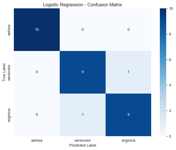
Probability Predictions
# Show probability predictions for first 5 test samples
print("Probability predictions (first 5 samples):")
prob_df = pd.DataFrame(
    y_pred_proba_lr[:5],
    columns=[f'P({name})' for name in iris.target_names]
)
prob_df['Predicted'] = [iris.target_names[i] for i in y_pred_lr[:5]]
prob_df['Actual'] = [iris.target_names[i] for i in y_test[:5]]
print(prob_df)
Probability predictions (first 5 samples):
P(setosa) P(versicolor) P(virginica) Predicted Actual
0 0.978818 0.021182 3.638218e-07 setosa setosa
1 0.003798 0.369220 6.269815e-01 virginica virginica
2 0.148799 0.842475 8.726064e-03 versicolor versicolor
3 0.095445 0.894619 9.936370e-03 versicolor versicolor
4 0.988493 0.011507 1.725496e-07 setosa setosa16.4 k-Nearest Neighbors (KNN)
What it is: KNN is a simple, instance-based learning algorithm that classifies new samples based on the majority class of their k nearest neighbors.
How it works: - Stores all training data - For a new sample, finds k closest training samples - Assigns the most common class among those neighbors
When to use: - ✅ Simple and intuitive - ✅ No training phase (lazy learning) - ✅ Works well with multi-class problems - ❌ Slow prediction for large datasets - ❌ Sensitive to irrelevant features
from sklearn.neighbors import KNeighborsClassifier

# Create and train the model
knn = KNeighborsClassifier(n_neighbors=5)
knn.fit(X_train_scaled, y_train)

# Make predictions
y_pred_knn = knn.predict(X_test_scaled)

# Evaluate
accuracy_knn = accuracy_score(y_test, y_pred_knn)
print(f"KNN Accuracy (k=5): {accuracy_knn:.4f}")
print("\nClassification Report:")
print(classification_report(y_test, y_pred_knn, target_names=iris.target_names))
KNN Accuracy (k=5): 0.9333
Classification Report:
precision recall f1-score support
setosa 1.00 1.00 1.00 10
versicolor 0.83 1.00 0.91 10
virginica 1.00 0.80 0.89 10
accuracy 0.93 30
macro avg 0.94 0.93 0.93 30
weighted avg 0.94 0.93 0.93 30
Finding the Optimal k
# Test different values of k
k_values = range(1, 21)
train_scores = []
test_scores = []

for k in k_values:
    knn_temp = KNeighborsClassifier(n_neighbors=k)
    knn_temp.fit(X_train_scaled, y_train)

    train_scores.append(knn_temp.score(X_train_scaled, y_train))
    test_scores.append(knn_temp.score(X_test_scaled, y_test))

# Plot results
plt.figure(figsize=(10, 6))
plt.plot(k_values, train_scores, label='Training Accuracy', marker='o')
plt.plot(k_values, test_scores, label='Test Accuracy', marker='s')
plt.xlabel('Number of Neighbors (k)')
plt.ylabel('Accuracy')
plt.title('KNN: Finding Optimal k')
plt.legend()
plt.grid(True)
plt.show()

best_k = k_values[np.argmax(test_scores)]
print(f"Best k value: {best_k} (Test Accuracy: {max(test_scores):.4f})")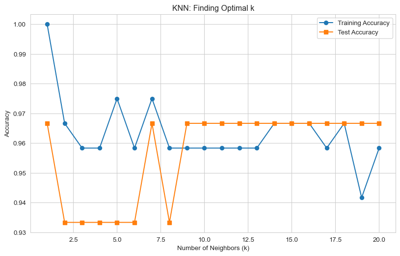
Best k value: 1 (Test Accuracy: 0.9667)Visualize Decision Boundaries (2D)
# Use only 2 features for visualization
X_train_2d = X_train_scaled[:, [2, 3]]  # petal length and width
X_test_2d = X_test_scaled[:, [2, 3]]

# Train KNN on 2D data
knn_2d = KNeighborsClassifier(n_neighbors=5)
knn_2d.fit(X_train_2d, y_train)

# Create mesh for decision boundary
h = 0.02
x_min, x_max = X_train_2d[:, 0].min() - 1, X_train_2d[:, 0].max() + 1
y_min, y_max = X_train_2d[:, 1].min() - 1, X_train_2d[:, 1].max() + 1
xx, yy = np.meshgrid(np.arange(x_min, x_max, h),
                     np.arange(y_min, y_max, h))

# Predict for each point in mesh
Z = knn_2d.predict(np.c_[xx.ravel(), yy.ravel()])
Z = Z.reshape(xx.shape)

# Plot
plt.figure(figsize=(10, 7))
plt.contourf(xx, yy, Z, alpha=0.3, cmap='viridis')
scatter = plt.scatter(X_train_2d[:, 0], X_train_2d[:, 1], c=y_train,
                     cmap='viridis', edgecolor='black', s=50)
plt.xlabel('Petal Length (scaled)')
plt.ylabel('Petal Width (scaled)')
plt.title('KNN Decision Boundaries (k=5)')
plt.colorbar(scatter)
plt.show()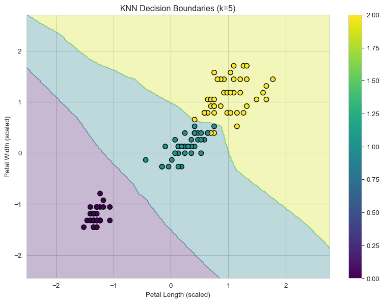
16.5 Support Vector Machines (SVM)
What it is: SVM finds the optimal hyperplane that maximally separates different classes by maximizing the margin between them.
How it works: - Finds the hyperplane with maximum margin - Uses “support vectors” (closest points to boundary) - Can use kernel trick for non-linear boundaries
When to use: - ✅ Effective in high-dimensional spaces - ✅ Works well with clear margin of separation - ✅ Versatile with different kernel functions - ❌ Slow for large datasets - ❌ Requires feature scaling
from sklearn.svm import SVC

# Create and train the model (RBF kernel)
svm = SVC(kernel='rbf', random_state=42, probability=True)
svm.fit(X_train_scaled, y_train)

# Make predictions
y_pred_svm = svm.predict(X_test_scaled)

# Evaluate
accuracy_svm = accuracy_score(y_test, y_pred_svm)
print(f"SVM Accuracy (RBF kernel): {accuracy_svm:.4f}")
print("\nClassification Report:")
print(classification_report(y_test, y_pred_svm, target_names=iris.target_names))
SVM Accuracy (RBF kernel): 0.9667
Classification Report:
precision recall f1-score support
setosa 1.00 1.00 1.00 10
versicolor 1.00 0.90 0.95 10
virginica 0.91 1.00 0.95 10
accuracy 0.97 30
macro avg 0.97 0.97 0.97 30
weighted avg 0.97 0.97 0.97 30
Comparing Different Kernels
# Test different kernels
kernels = ['linear', 'rbf', 'poly', 'sigmoid']
kernel_scores = {}

for kernel in kernels:
    svm_temp = SVC(kernel=kernel, random_state=42)
    svm_temp.fit(X_train_scaled, y_train)
    score = svm_temp.score(X_test_scaled, y_test)
    kernel_scores[kernel] = score
    print(f"{kernel.upper()} kernel: {score:.4f}")

# Visualize kernel comparison
plt.figure(figsize=(10, 6))
plt.bar(kernel_scores.keys(), kernel_scores.values(), color='skyblue', edgecolor='black')
plt.ylabel('Accuracy')
plt.xlabel('Kernel Type')
plt.title('SVM Performance with Different Kernels')
plt.ylim([0, 1.0])
for i, (kernel, score) in enumerate(kernel_scores.items()):
    plt.text(i, score + 0.02, f'{score:.3f}', ha='center', va='bottom')
plt.show()
LINEAR kernel: 1.0000
RBF kernel: 0.9667
POLY kernel: 0.9000
SIGMOID kernel: 0.9000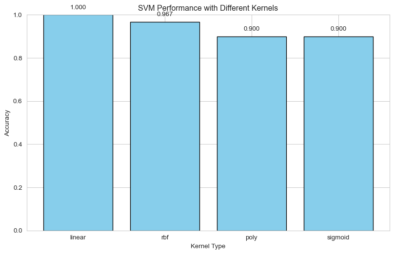
SVM Decision Boundary (2D)
# Train SVM on 2D data
svm_2d = SVC(kernel='rbf', random_state=42)
svm_2d.fit(X_train_2d, y_train)

# Create mesh
Z_svm = svm_2d.predict(np.c_[xx.ravel(), yy.ravel()])
Z_svm = Z_svm.reshape(xx.shape)

# Plot
plt.figure(figsize=(10, 7))
plt.contourf(xx, yy, Z_svm, alpha=0.3, cmap='viridis')
scatter = plt.scatter(X_train_2d[:, 0], X_train_2d[:, 1], c=y_train,
                     cmap='viridis', edgecolor='black', s=50)

# Highlight support vectors
support_vectors = svm_2d.support_vectors_
plt.scatter(support_vectors[:, 0], support_vectors[:, 1],
           s=200, facecolors='none', edgecolors='red', linewidths=2,
           label='Support Vectors')

plt.xlabel('Petal Length (scaled)')
plt.ylabel('Petal Width (scaled)')
plt.title('SVM Decision Boundaries (RBF Kernel)')
plt.colorbar(scatter)
plt.legend()
plt.show()

print(f"Number of support vectors: {len(support_vectors)}")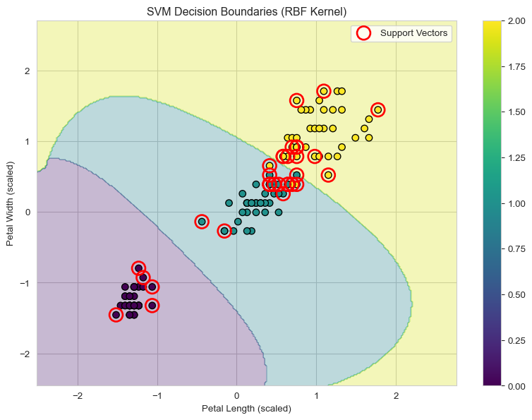
Number of support vectors: 3216.6 Decision Trees
What it is: Decision Trees learn a series of if-then-else rules from features to make predictions. Think of it as a flowchart.
How it works: - Recursively splits data based on feature thresholds - Creates tree structure with decision nodes and leaf nodes - Each leaf represents a class prediction
When to use: - ✅ Easy to interpret and visualize - ✅ Requires little data preprocessing - ✅ Handles both numerical and categorical data - ✅ Captures non-linear relationships - ❌ Prone to overfitting - ❌ Can be unstable (small data changes affect tree)
from sklearn.tree import DecisionTreeClassifier

# Create and train the model
dt = DecisionTreeClassifier(random_state=42, max_depth=3)
dt.fit(X_train, y_train)  # Decision trees don't require scaling

# Make predictions
y_pred_dt = dt.predict(X_test)

# Evaluate
accuracy_dt = accuracy_score(y_test, y_pred_dt)
print(f"Decision Tree Accuracy: {accuracy_dt:.4f}")
print("\nClassification Report:")
print(classification_report(y_test, y_pred_dt, target_names=iris.target_names))
Decision Tree Accuracy: 0.9667
Classification Report:
precision recall f1-score support
setosa 1.00 1.00 1.00 10
versicolor 1.00 0.90 0.95 10
virginica 0.91 1.00 0.95 10
accuracy 0.97 30
macro avg 0.97 0.97 0.97 30
weighted avg 0.97 0.97 0.97 30
Visualize the Decision Tree
from sklearn.tree import plot_tree

# Plot the tree
plt.figure(figsize=(20, 10))
plot_tree(dt,
          feature_names=iris.feature_names,
          class_names=iris.target_names,
          filled=True,
          rounded=True,
          fontsize=10)
plt.title('Decision Tree Visualization')
plt.show()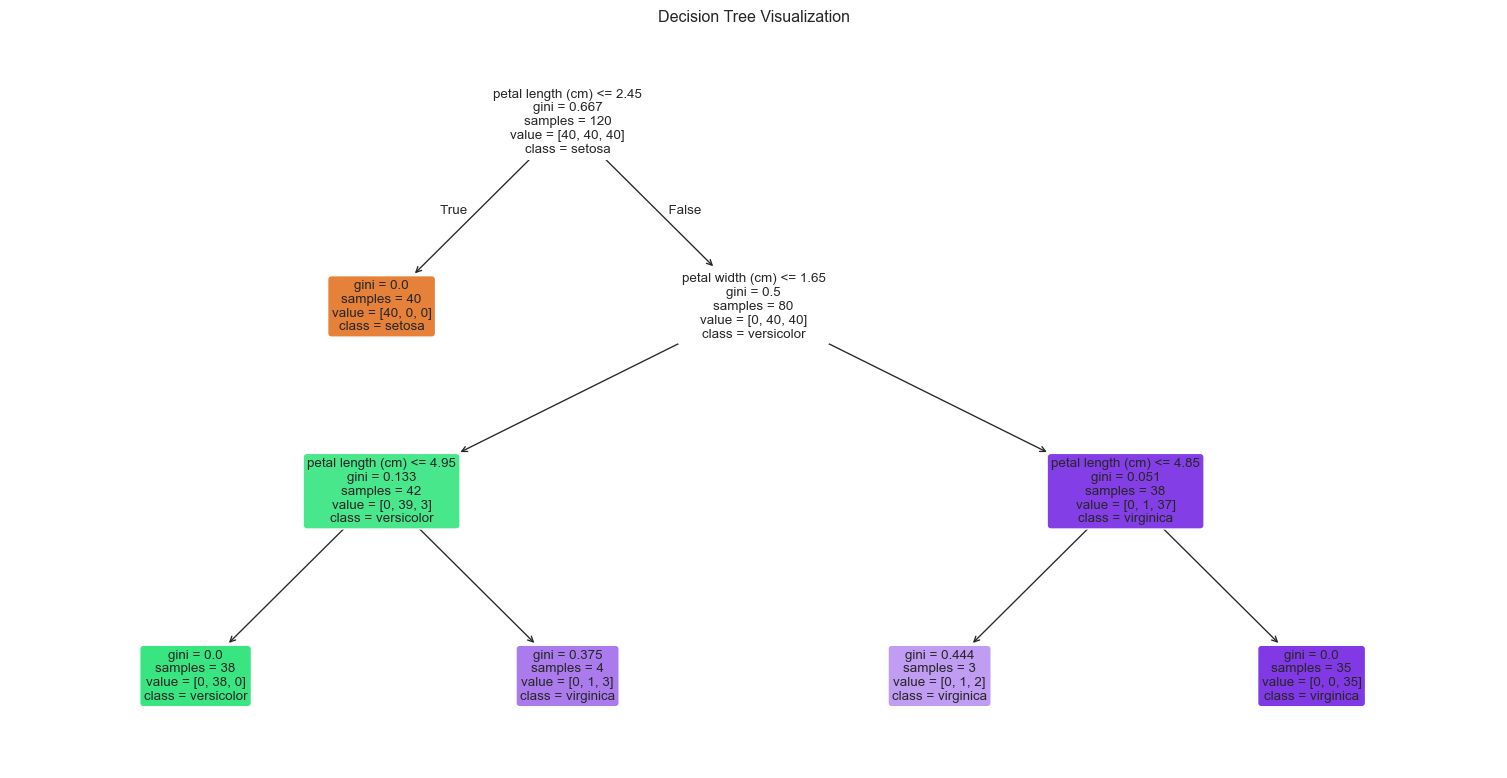
Feature Importance
# Get feature importances
feature_importance = pd.DataFrame({
    'feature': iris.feature_names,
    'importance': dt.feature_importances_
}).sort_values('importance', ascending=False)

print("Feature Importances:")
print(feature_importance)

# Visualize
plt.figure(figsize=(10, 6))
plt.barh(feature_importance['feature'], feature_importance['importance'], color='green', alpha=0.7)
plt.xlabel('Importance')
plt.ylabel('Feature')
plt.title('Decision Tree: Feature Importance')
plt.gca().invert_yaxis()
plt.show()
Feature Importances:
feature importance
2 petal length (cm) 0.579077
3 petal width (cm) 0.420923
0 sepal length (cm) 0.000000
1 sepal width (cm) 0.000000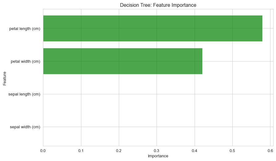
Effect of Tree Depth
# Test different max_depth values
depths = range(1, 11)
train_scores_dt = []
test_scores_dt = []

for depth in depths:
    dt_temp = DecisionTreeClassifier(max_depth=depth, random_state=42)
    dt_temp.fit(X_train, y_train)

    train_scores_dt.append(dt_temp.score(X_train, y_train))
    test_scores_dt.append(dt_temp.score(X_test, y_test))

# Plot
plt.figure(figsize=(10, 6))
plt.plot(depths, train_scores_dt, label='Training Accuracy', marker='o')
plt.plot(depths, test_scores_dt, label='Test Accuracy', marker='s')
plt.xlabel('Max Depth')
plt.ylabel('Accuracy')
plt.title('Decision Tree: Effect of Max Depth on Performance')
plt.legend()
plt.grid(True)
plt.show()

print("Notice: Training accuracy keeps increasing, but test accuracy plateaus")
print("This is a sign of overfitting when tree is too deep!")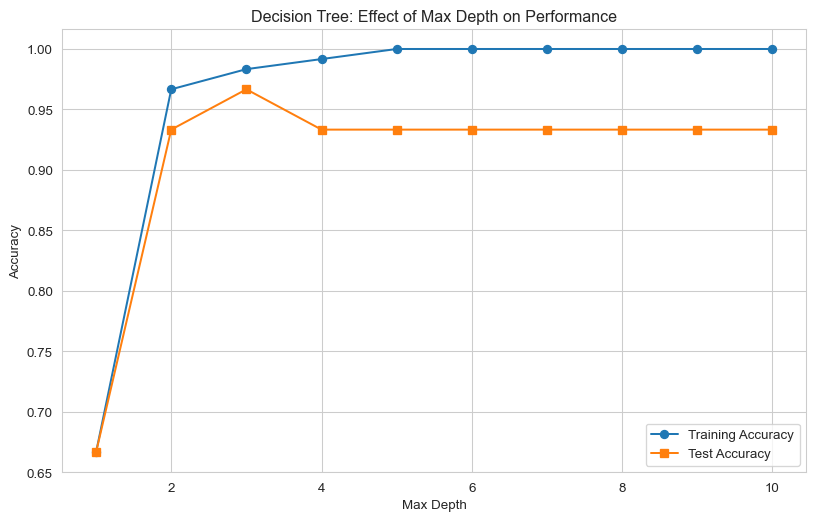
Notice: Training accuracy keeps increasing, but test accuracy plateaus
This is a sign of overfitting when tree is too deep!
16.7 Model Comparison
Let’s compare all four models:
# Create a comparison DataFrame
results = pd.DataFrame({
    'Model': ['Logistic Regression', 'KNN', 'SVM', 'Decision Tree'],
    'Accuracy': [accuracy_lr, accuracy_knn, accuracy_svm, accuracy_dt]
}).sort_values('Accuracy', ascending=False)

print("Model Comparison:")
print(results)
print(f"\nBest Model: {results.iloc[0]['Model']} ({results.iloc[0]['Accuracy']:.4f})")

# Visualize comparison
plt.figure(figsize=(10, 6))
colors = ['#FF6B6B', '#4ECDC4', '#45B7D1', '#96CEB4']
bars = plt.bar(results['Model'], results['Accuracy'], color=colors, edgecolor='black', linewidth=1.5)
plt.ylabel('Accuracy')
plt.xlabel('Model')
plt.title('Classification Model Comparison on Iris Dataset')
plt.ylim([0.9, 1.0])
plt.xticks(rotation=15, ha='right')

for bar in bars:
    height = bar.get_height()
    plt.text(bar.get_x() + bar.get_width()/2., height,
             f'{height:.4f}',
             ha='center', va='bottom', fontweight='bold')
plt.tight_layout()
plt.show()
Model Comparison:
Model Accuracy
2 SVM 0.966667
3 Decision Tree 0.966667
0 Logistic Regression 0.933333
1 KNN 0.933333
Best Model: SVM (0.9667)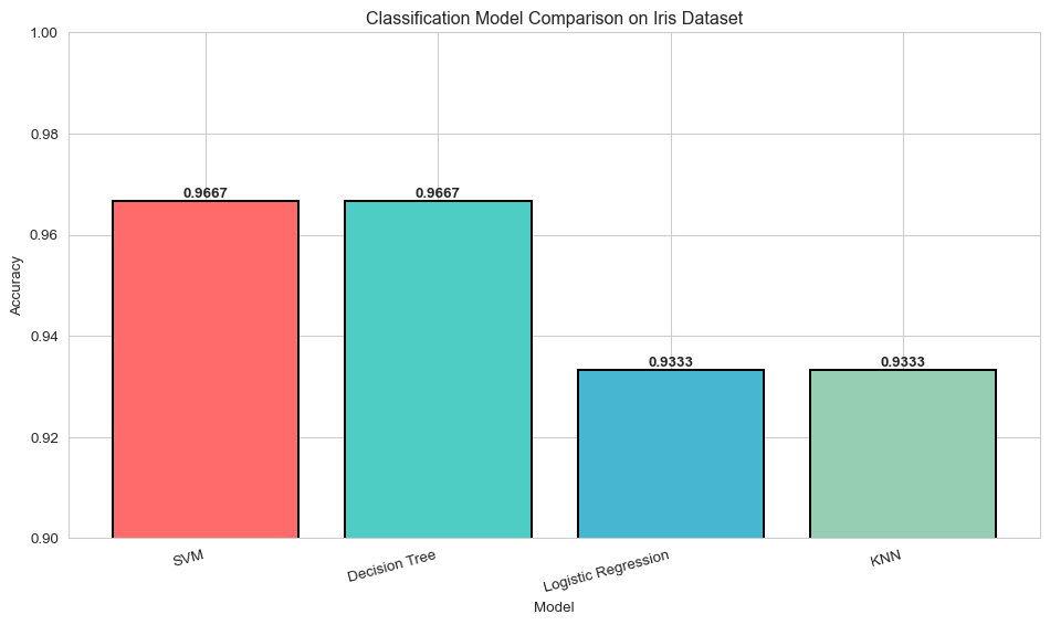
16.8 Real-World Example: Email Spam Detection
Let’s create a simple spam/not spam classifier:
from sklearn.feature_extraction.text import CountVectorizer

# Sample email dataset
emails = [
    "Win a free iPhone now! Click here!",
    "Meeting scheduled for tomorrow at 10am",
    "Congratulations! You've won $1,000,000",
    "Please review the attached document",
    "Get rich quick! Limited time offer!",
    "Lunch with the team next week?",
    "Your package has been delivered",
    "URGENT: Verify your account immediately",
    "Project deadline is Friday",
    "Buy now and save 90%! Act fast!"
]

labels = [1, 0, 1, 0, 1, 0, 0, 1, 0, 1]  # 1=spam, 0=not spam

# Convert text to numerical features
vectorizer = CountVectorizer()
X_emails = vectorizer.fit_transform(emails)

print(f"Email features shape: {X_emails.shape}")
print(f"Vocabulary size: {len(vectorizer.vocabulary_)}")

# Train a logistic regression model
spam_model = LogisticRegression(random_state=42)
spam_model.fit(X_emails, labels)

# Test on new emails
new_emails = [
    "Team meeting at 2pm in conference room B",
    "You've been selected for a FREE prize!"
]

X_new = vectorizer.transform(new_emails)
predictions = spam_model.predict(X_new)
probabilities = spam_model.predict_proba(X_new)

for email, pred, prob in zip(new_emails, predictions, probabilities):
    label = "SPAM" if pred == 1 else "NOT SPAM"
    confidence = prob[pred] * 100
    print(f"\nEmail: '{email}'")
    print(f"Prediction: {label} (Confidence: {confidence:.1f}%)")
Email features shape: (10, 52)
Vocabulary size: 52
Email: 'Team meeting at 2pm in conference room B'
Prediction: NOT SPAM (Confidence: 67.4%)
Email: 'You've been selected for a FREE prize!'
Prediction: SPAM (Confidence: 50.4%)16.9 Best Practices and Tips
- Always Split Your Data
# Good practice: train/test split
from sklearn.model_selection import train_test_split

X_train, X_test, y_train, y_test = train_test_split(
    X, y, test_size=0.2, random_state=42, stratify=y
)- Use Cross-Validation
from sklearn.model_selection import cross_val_score

# Evaluate model using 5-fold cross-validation
log_reg_cv = LogisticRegression(random_state=42, max_iter=200)
cv_scores = cross_val_score(log_reg_cv, X_train_scaled, y_train, cv=5)

print(f"Cross-validation scores: {cv_scores}")
print(f"Mean accuracy: {cv_scores.mean():.4f} (+/- {cv_scores.std() * 2:.4f})")
Cross-validation scores: [0.91666667 0.95833333 0.95833333 0.95833333 1. ]
Mean accuracy: 0.9583 (+/- 0.0527)- Handle Imbalanced Classes
# For imbalanced datasets, use class_weight='balanced'
log_reg_balanced = LogisticRegression(class_weight='balanced', random_state=42)

# Or use stratified sampling
X_train_strat, X_test_strat, y_train_strat, y_test_strat = train_test_split(
    X, y, test_size=0.2, random_state=42, stratify=y  # Maintains class distribution
)- Hyperparameter Tuning
from sklearn.model_selection import GridSearchCV

# Define parameter grid
param_grid = {
    'C': [0.1, 1, 10],
    'penalty': ['l1', 'l2'],
    'solver': ['liblinear']
}

# Grid search
grid_search = GridSearchCV(LogisticRegression(random_state=42),
                          param_grid, cv=5, scoring='accuracy')
grid_search.fit(X_train_scaled, y_train)

print(f"Best parameters: {grid_search.best_params_}")
print(f"Best cross-validation score: {grid_search.best_score_:.4f}")
Best parameters: {'C': 10, 'penalty': 'l1', 'solver': 'liblinear'}
Best cross-validation score: 0.958316.10 Quick Reference Guide
| Model | Pros | Cons | When to Use |
|---|---|---|---|
| Logistic Regression | Fast, interpretable, probabilistic | Assumes linear decision boundary | Good baseline, linearly separable data |
| KNN | Simple, no training, non-linear | Slow prediction, sensitive to scale | Small datasets, unknown pattern |
| SVM | Effective in high dimensions, versatile | Slow on large data, needs scaling | Clear margins, high-dimensional data |
| Decision Trees | Interpretable, no scaling needed | Overfitting, unstable | Need interpretability, mixed data types |
16.11 Common Parameters
Logistic Regression
LogisticRegression(
    C=1.0,              # Regularization strength (smaller = stronger)
    penalty='l2',       # 'l1', 'l2', 'elasticnet', 'none'
    solver='lbfgs',     # 'newton-cg', 'lbfgs', 'liblinear', 'sag', 'saga'
    max_iter=100        # Maximum iterations
)
KNN
KNeighborsClassifier(
    n_neighbors=5,      # Number of neighbors
    weights='uniform',  # 'uniform' or 'distance'
    metric='minkowski', # Distance metric
    p=2                 # Power parameter (1=manhattan, 2=euclidean)
)
SVM
SVC(
    C=1.0,             # Regularization parameter
    kernel='rbf',      # 'linear', 'poly', 'rbf', 'sigmoid'
    gamma='scale',     # Kernel coefficient
    probability=False  # Enable probability estimates (slower)
)
Decision Tree
DecisionTreeClassifier(
    max_depth=None,         # Maximum tree depth
    min_samples_split=2,    # Min samples to split node
    min_samples_leaf=1,     # Min samples in leaf
    criterion='gini'        # 'gini' or 'entropy'
)
16.12 Practice Exercises
Exercise 1: Binary Classification
Create a binary classifier to distinguish between two iris species:
# Filter for only setosa (0) and versicolor (1)
mask = y < 2
X_binary = X[mask]
y_binary = y[mask]

# Split the data
# Train a logistic regression model
# Evaluate its performance
Exercise 2: Optimize KNN
Find the best k value and distance metric for KNN:
# Try k values from 1 to 20
# Try different distance metrics: 'euclidean', 'manhattan', 'chebyshev'
# Plot the results
Exercise 3: Compare Models
Use a different dataset and compare all four models:
from sklearn.datasets import load_breast_cancer

# Load breast cancer dataset
data = load_breast_cancer()
# Preprocess and split
# Train all four models
# Compare accuracies
16.13 Solutions
Solution 1:
Click to show solution
# Binary classification
mask = y < 2
X_binary = X[mask]
y_binary = y[mask]

X_train_bin, X_test_bin, y_train_bin, y_test_bin = train_test_split(
    X_binary, y_binary, test_size=0.2, random_state=42
)

# Scale features
scaler_bin = StandardScaler()
X_train_bin_scaled = scaler_bin.fit_transform(X_train_bin)
X_test_bin_scaled = scaler_bin.transform(X_test_bin)

# Train model
log_reg_bin = LogisticRegression(random_state=42)
log_reg_bin.fit(X_train_bin_scaled, y_train_bin)

# Evaluate
y_pred_bin = log_reg_bin.predict(X_test_bin_scaled)
print(f"Binary Classification Accuracy: {accuracy_score(y_test_bin, y_pred_bin):.4f}")
Binary Classification Accuracy: 1.0000Solution 2:
Click to show solution
# Optimize KNN
k_range = range(1, 21)
metrics = ['euclidean', 'manhattan', 'chebyshev']
results_dict = {}

for metric in metrics:
    scores = []
    for k in k_range:
        knn_opt = KNeighborsClassifier(n_neighbors=k, metric=metric)
        knn_opt.fit(X_train_scaled, y_train)
        scores.append(knn_opt.score(X_test_scaled, y_test))
    results_dict[metric] = scores

# Plot
plt.figure(figsize=(10, 6))
for metric, scores in results_dict.items():
    plt.plot(k_range, scores, marker='o', label=metric)
plt.xlabel('k')
plt.ylabel('Accuracy')
plt.title('KNN Optimization: k vs Distance Metric')
plt.legend()
plt.grid(True)
plt.show()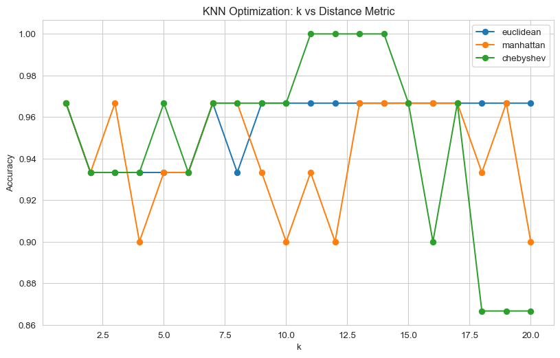
16.14 Key Takeaways
- Choose the right model for your problem:
- Start with Logistic Regression as baseline
- Use KNN for small datasets with no clear pattern
- Use SVM for high-dimensional data with clear separation
- Use Decision Trees when interpretability is crucial
- Always preprocess your data:
- Split into train/test sets
- Scale features (especially for KNN, SVM, Logistic Regression)
- Handle missing values and outliers
- Evaluate properly:
- Use cross-validation, not just single train/test split
- Look at multiple metrics (accuracy, precision, recall, F1)
- Check confusion matrix for class-specific performance
- Avoid overfitting:
- Use regularization (C parameter in Logistic Regression, SVM)
- Limit tree depth in Decision Trees
- Use cross-validation to detect overfitting
16.15 Next Steps
Now that you understand classification, explore: - Ensemble Methods: Random Forests, Gradient Boosting - Regression: Predicting continuous values - Clustering: Unsupervised learning - Feature Engineering: Creating better features - Model Deployment: Putting models into production
Keep practicing and happy classifying!