import matplotlib.pyplot as plt

# Data
x = [1, 2, 3, 4, 5]
y = [2, 4, 6, 8, 10]

# Create plot
plt.plot(x, y)
plt.title("My First Plot")
plt.xlabel("X-axis")
plt.ylabel("Y-axis")
plt.show()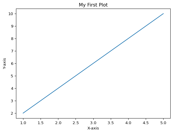
Matplotlib is the most popular plotting library in Python. It provides a flexible way to create static, animated, and interactive visualizations. This tutorial will introduce you to the fundamentals of creating charts and graphs with Matplotlib.
First, you need to install matplotlib if you haven’t already:
pip install matplotlibMatplotlib has two main interfaces: - pyplot: A MATLAB-like interface (simpler, procedural) - Object-oriented interface: More control and flexibility
We’ll focus on pyplot for beginners, using the common alias plt.
Let’s create a simple line plot:
import matplotlib.pyplot as plt
# Data
x = [1, 2, 3, 4, 5]
y = [2, 4, 6, 8, 10]
# Create plot
plt.plot(x, y)
plt.title("My First Plot")
plt.xlabel("X-axis")
plt.ylabel("Y-axis")
plt.show()
Line plots are great for showing trends over time:
import matplotlib.pyplot as plt
import numpy as np

# Generate data
x = np.linspace(0, 10, 100)
y = np.sin(x)

# Create line plot
plt.plot(x, y, color='blue', linewidth=2, label='sin(x)')
plt.title("Sine Wave")
plt.xlabel("X")
plt.ylabel("Y")
plt.legend()
plt.grid(True)
plt.show()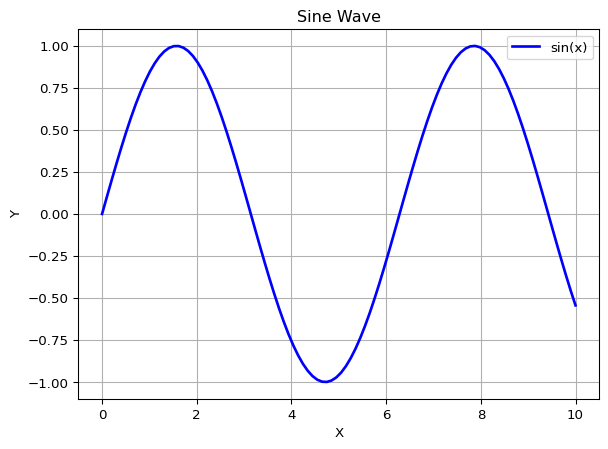
Scatter plots show relationships between two variables:
# Generate random data
np.random.seed(42)
x = np.random.randn(50)
y = np.random.randn(50)
colors = np.random.rand(50)
sizes = 1000 * np.random.rand(50)

# Create scatter plot
plt.scatter(x, y, c=colors, s=sizes, alpha=0.5, cmap='viridis')
plt.colorbar()
plt.title("Scatter Plot Example")
plt.xlabel("X values")
plt.ylabel("Y values")
plt.show()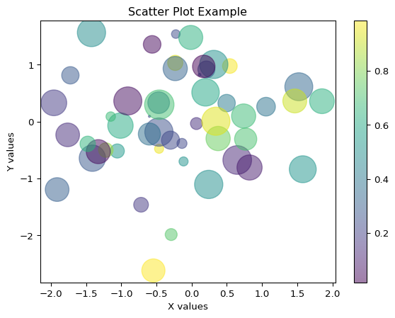
Bar charts are useful for comparing categories:
# Data
categories = ['Python', 'Java', 'C++', 'JavaScript', 'Go']
values = [85, 70, 60, 75, 55]

# Create bar chart
plt.bar(categories, values, color='skyblue', edgecolor='navy')
plt.title("Programming Language Popularity")
plt.xlabel("Language")
plt.ylabel("Popularity Score")
plt.xticks(rotation=45)
plt.tight_layout()
plt.show()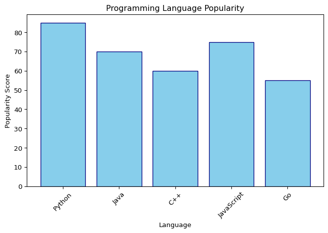
Histograms show the distribution of data:
# Generate random data
data = np.random.randn(1000)

# Create histogram
plt.hist(data, bins=30, color='green', alpha=0.7, edgecolor='black')
plt.title("Normal Distribution Histogram")
plt.xlabel("Value")
plt.ylabel("Frequency")
plt.grid(axis='y', alpha=0.3)
plt.show()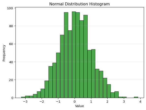
Pie charts show proportions:
# Data
labels = ['Python', 'JavaScript', 'Java', 'C++', 'Others']
sizes = [35, 25, 20, 10, 10]
colors = ['#ff9999', '#66b3ff', '#99ff99', '#ffcc99', '#ff99cc']
explode = (0.1, 0, 0, 0, 0)  # explode the 1st slice

# Create pie chart
plt.pie(sizes, explode=explode, labels=labels, colors=colors,
        autopct='%1.1f%%', shadow=True, startangle=90)
plt.axis('equal')
plt.title("Programming Language Usage")
plt.show()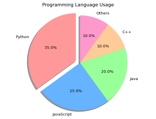
x = np.linspace(0, 10, 100)

# Different line styles and colors
plt.plot(x, np.sin(x), 'r-', label='sin(x) - solid red')
plt.plot(x, np.cos(x), 'b--', label='cos(x) - dashed blue')
plt.plot(x, np.sin(x) * np.cos(x), 'g:', linewidth=3, label='sin(x)*cos(x) - dotted green')

plt.title("Multiple Line Styles")
plt.xlabel("X")
plt.ylabel("Y")
plt.legend()
plt.grid(True, alpha=0.3)
plt.show()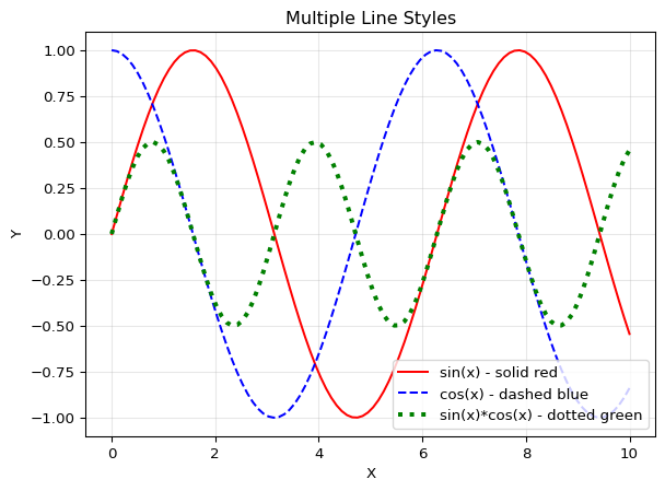
# Create figure with custom size
plt.figure(figsize=(10, 6), dpi=100)

x = np.linspace(0, 2*np.pi, 100)
plt.plot(x, np.sin(x), label='sin(x)')
plt.plot(x, np.cos(x), label='cos(x)')

plt.title("Custom Figure Size", fontsize=16)
plt.xlabel("X", fontsize=12)
plt.ylabel("Y", fontsize=12)
plt.legend(fontsize=10)
plt.grid(True)
plt.show()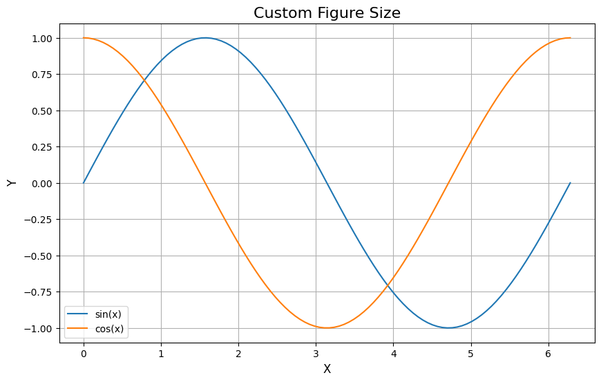
Create multiple plots in one figure:
# Create 2x2 grid of subplots
fig, axes = plt.subplots(2, 2, figsize=(12, 10))

x = np.linspace(0, 5, 100)

# Plot 1: Line plot
axes[0, 0].plot(x, x**2)
axes[0, 0].set_title('Quadratic')
axes[0, 0].set_xlabel('x')
axes[0, 0].set_ylabel('x²')
axes[0, 0].grid(True)

# Plot 2: Scatter plot
axes[0, 1].scatter(x, np.sin(x), c='red', alpha=0.5)
axes[0, 1].set_title('Scatter')
axes[0, 1].set_xlabel('x')
axes[0, 1].set_ylabel('sin(x)')
axes[0, 1].grid(True)

# Plot 3: Bar chart
axes[1, 0].bar(['A', 'B', 'C', 'D'], [3, 7, 2, 5], color='green')
axes[1, 0].set_title('Bar Chart')
axes[1, 0].set_ylabel('Values')

# Plot 4: Histogram
axes[1, 1].hist(np.random.randn(1000), bins=20, color='purple', alpha=0.7)
axes[1, 1].set_title('Histogram')
axes[1, 1].set_xlabel('Value')
axes[1, 1].set_ylabel('Frequency')

plt.tight_layout()
plt.show()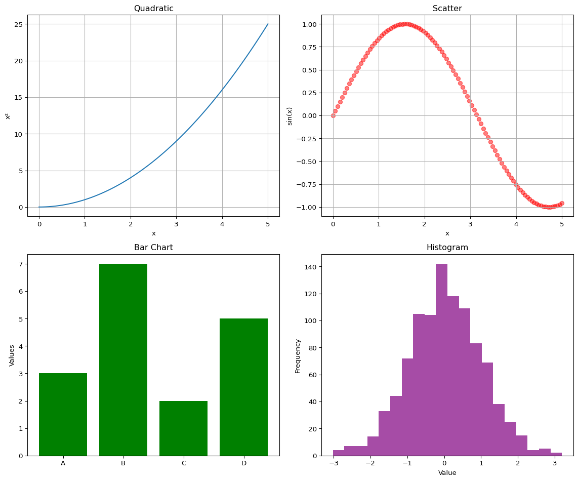
You can save your plots in various formats:
# Create a simple plot
x = np.linspace(0, 10, 100)
y = np.sin(x)

plt.figure(figsize=(8, 6))
plt.plot(x, y)
plt.title("Saved Figure Example")
plt.xlabel("X")
plt.ylabel("sin(X)")
plt.grid(True)

# Save in different formats
# plt.savefig('my_plot.png', dpi=300, bbox_inches='tight')
# plt.savefig('my_plot.pdf', bbox_inches='tight')
# plt.savefig('my_plot.svg', bbox_inches='tight')

plt.show()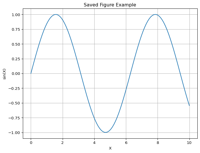
Let’s create a more complex visualization:
# Simulated monthly temperature data
months = ['Jan', 'Feb', 'Mar', 'Apr', 'May', 'Jun',
          'Jul', 'Aug', 'Sep', 'Oct', 'Nov', 'Dec']
temp_2022 = [5, 7, 12, 15, 20, 25, 28, 27, 23, 17, 10, 6]
temp_2023 = [6, 8, 13, 16, 21, 26, 29, 28, 24, 18, 11, 7]

# Create figure
fig, (ax1, ax2) = plt.subplots(1, 2, figsize=(14, 5))

# Line plot comparison
ax1.plot(months, temp_2022, marker='o', linewidth=2, label='2022')
ax1.plot(months, temp_2023, marker='s', linewidth=2, label='2023')
ax1.set_title('Monthly Temperature Comparison', fontsize=14, fontweight='bold')
ax1.set_xlabel('Month', fontsize=12)
ax1.set_ylabel('Temperature (°C)', fontsize=12)
ax1.legend()
ax1.grid(True, alpha=0.3)

# Bar chart of average temperatures
avg_temps = [(t1 + t2) / 2 for t1, t2 in zip(temp_2022, temp_2023)]
colors_bar = ['blue' if t < 15 else 'orange' if t < 25 else 'red' for t in avg_temps]
ax2.bar(months, avg_temps, color=colors_bar, alpha=0.7, edgecolor='black')
ax2.set_title('Average Monthly Temperature', fontsize=14, fontweight='bold')
ax2.set_xlabel('Month', fontsize=12)
ax2.set_ylabel('Avg Temperature (°C)', fontsize=12)
ax2.axhline(y=15, color='gray', linestyle='--', alpha=0.5, label='15°C threshold')
ax2.axhline(y=25, color='gray', linestyle='--', alpha=0.5, label='25°C threshold')
ax2.legend()
ax2.grid(axis='y', alpha=0.3)

plt.tight_layout()
plt.show()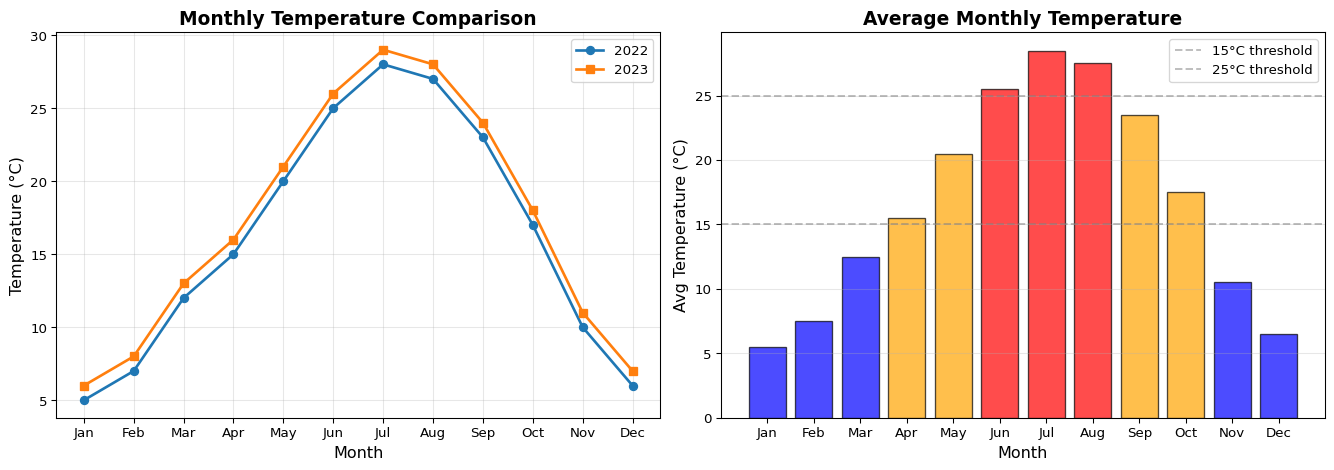
| Function | Description |
|---|---|
plt.plot() |
Create a line plot |
plt.scatter() |
Create a scatter plot |
plt.bar() |
Create a bar chart |
plt.hist() |
Create a histogram |
plt.pie() |
Create a pie chart |
plt.xlabel() |
Set x-axis label |
plt.ylabel() |
Set y-axis label |
plt.title() |
Set plot title |
plt.legend() |
Add legend |
plt.grid() |
Add grid lines |
plt.show() |
Display the plot |
plt.savefig() |
Save the plot to file |
plt.figure() |
Create a new figure |
plt.subplot() |
Create subplots |
pltfigsize for better readabilityplt.tight_layout() to prevent label overlapplt.style.use('style_name'))Create a line plot showing temperature changes throughout a week.
Create a bar chart showing grades of 5 students in different subjects.
Generate 1000 random numbers and create a histogram to visualize the distribution.
Create a subplot with 4 different plot types showing the same x values.
# Temperature plot for a week
days = ['Mon', 'Tue', 'Wed', 'Thu', 'Fri', 'Sat', 'Sun']
temps = [72, 68, 75, 80, 77, 82, 79]

plt.figure(figsize=(10, 6))
plt.plot(days, temps, marker='o', linestyle='-', color='orange', linewidth=2, markersize=8)
plt.title('Weekly Temperature Changes', fontsize=14, fontweight='bold')
plt.xlabel('Day of Week')
plt.ylabel('Temperature (°F)')
plt.grid(True, linestyle='--', alpha=0.7)
plt.tight_layout()
plt.show()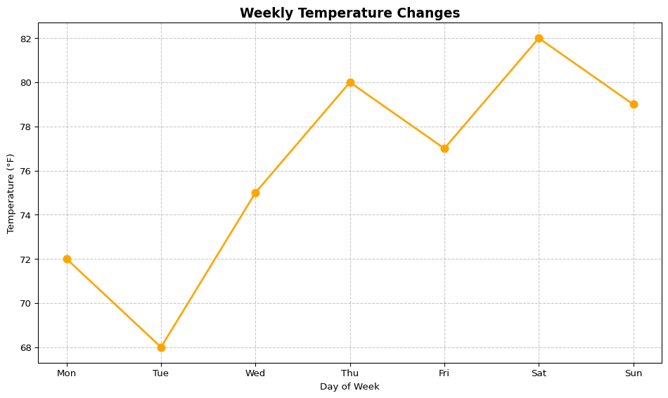
# Student grades bar chart
students = ['Alice', 'Bob', 'Charlie', 'Diana', 'Eve']
math_scores = [85, 90, 78, 92, 88]
science_scores = [88, 85, 92, 90, 87]

x = np.arange(len(students))
width = 0.35

fig, ax = plt.subplots(figsize=(10, 6))
bars1 = ax.bar(x - width/2, math_scores, width, label='Math', color='steelblue')
bars2 = ax.bar(x + width/2, science_scores, width, label='Science', color='coral')

ax.set_xlabel('Students')
ax.set_ylabel('Scores')
ax.set_title('Student Grades by Subject')
ax.set_xticks(x)
ax.set_xticklabels(students)
ax.legend()
ax.set_ylim(0, 100)
plt.tight_layout()
plt.show()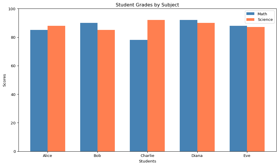
# Histogram of random numbers
np.random.seed(42)
data = np.random.randn(1000)

plt.figure(figsize=(10, 6))
plt.hist(data, bins=30, edgecolor='black', alpha=0.7, color='skyblue')
plt.title('Distribution of 1000 Random Numbers', fontsize=14)
plt.xlabel('Value')
plt.ylabel('Frequency')
plt.axvline(data.mean(), color='red', linestyle='--', label=f'Mean: {data.mean():.2f}')
plt.legend()
plt.tight_layout()
plt.show()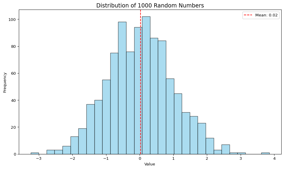
# Subplots with 4 different plot types
x = np.linspace(0, 10, 50)
y = np.sin(x)

fig, axes = plt.subplots(2, 2, figsize=(12, 10))

# Line plot
axes[0, 0].plot(x, y, 'b-', linewidth=2)
axes[0, 0].set_title('Line Plot')
axes[0, 0].set_xlabel('x')
axes[0, 0].set_ylabel('sin(x)')
axes[0, 0].grid(True)

# Scatter plot
axes[0, 1].scatter(x, y, c=y, cmap='viridis', s=50)
axes[0, 1].set_title('Scatter Plot')
axes[0, 1].set_xlabel('x')
axes[0, 1].set_ylabel('sin(x)')

# Bar plot (using first 10 values)
axes[1, 0].bar(x[:10], y[:10], color='coral', edgecolor='black')
axes[1, 0].set_title('Bar Plot')
axes[1, 0].set_xlabel('x')
axes[1, 0].set_ylabel('sin(x)')

# Area plot
axes[1, 1].fill_between(x, y, alpha=0.5, color='green')
axes[1, 1].plot(x, y, 'g-', linewidth=2)
axes[1, 1].set_title('Area Plot')
axes[1, 1].set_xlabel('x')
axes[1, 1].set_ylabel('sin(x)')

plt.suptitle('Comparison of Plot Types', fontsize=14, fontweight='bold')
plt.tight_layout()
plt.show()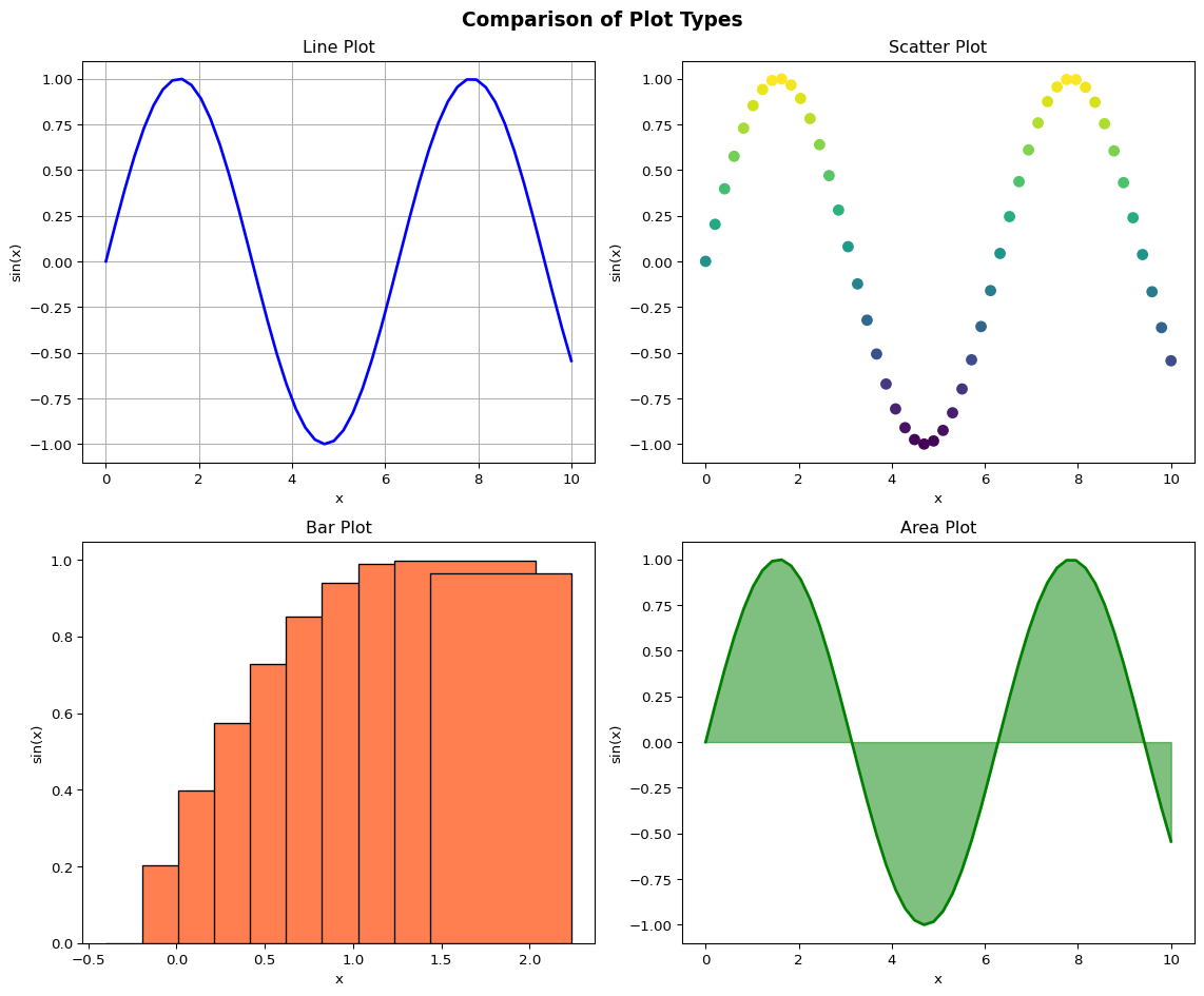
Matplotlib is a powerful library for data visualization in Python. This tutorial covered:
Practice these concepts with your own data to become proficient in data visualization!
Happy plotting!