import seaborn as sns
import matplotlib.pyplot as plt
import pandas as pd
import numpy as np

# Set the default theme
sns.set_theme()

# Display plots inline
%matplotlib inline15 Seaborn: Statistical Visualization
15.1 Welcome to Seaborn!
Seaborn is a powerful Python data visualization library built on top of Matplotlib. It makes creating beautiful, informative statistical graphics simple and intuitive. This guide will teach you the fundamentals of Seaborn for creating professional visualizations.
15.2 What is Seaborn?
Seaborn provides: - High-level interface for attractive statistical graphics - Built-in themes for professional-looking plots - Tools for visualizing distributions and relationships - Integration with pandas DataFrames - Statistical estimation and visualization
15.3 Installation and Setup
First, let’s import the libraries we’ll need:
15.4 Loading Sample Data
Seaborn comes with several built-in datasets perfect for learning:
# Load the tips dataset
tips = sns.load_dataset('tips')

# Display the first few rows
print(tips.head())
print(f"\nDataset shape: {tips.shape}")
print(f"Columns: {tips.columns.tolist()}")
total_bill tip sex smoker day time size
0 16.99 1.01 Female No Sun Dinner 2
1 10.34 1.66 Male No Sun Dinner 3
2 21.01 3.50 Male No Sun Dinner 3
3 23.68 3.31 Male No Sun Dinner 2
4 24.59 3.61 Female No Sun Dinner 4
Dataset shape: (244, 7)
Columns: ['total_bill', 'tip', 'sex', 'smoker', 'day', 'time', 'size']15.5 Basic Plots
1. Scatter Plot - Visualizing Relationships
Scatter plots show the relationship between two numerical variables:
# Create a simple scatter plot
plt.figure(figsize=(10, 6))
sns.scatterplot(data=tips, x='total_bill', y='tip')
plt.title('Relationship between Total Bill and Tip')
plt.show()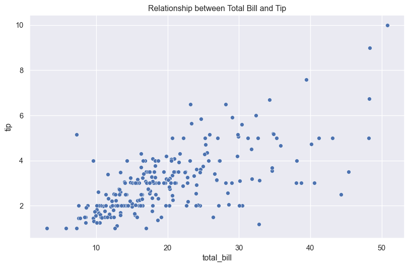
Adding more dimensions with color and size:
# Color by category, size by party size
plt.figure(figsize=(10, 6))
sns.scatterplot(data=tips, x='total_bill', y='tip',
                hue='time', size='size', sizes=(50, 200))
plt.title('Tips with Time of Day and Party Size')
plt.show()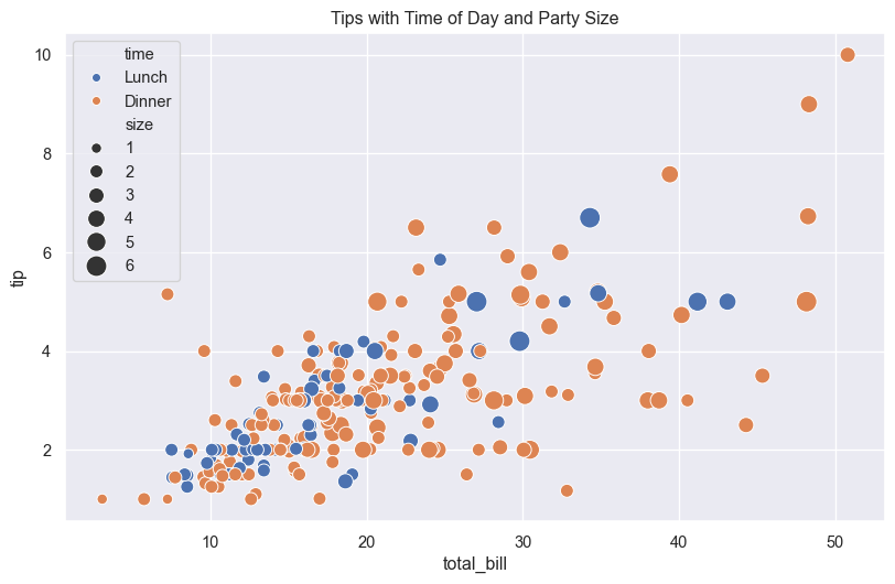
2. Line Plot - Showing Trends
Line plots are great for time series or continuous data:
# Load the flights dataset
flights = sns.load_dataset('flights')

# Filter for a specific month
may_flights = flights[flights['month'] == 'May']

plt.figure(figsize=(10, 6))
sns.lineplot(data=may_flights, x='year', y='passengers')
plt.title('Passenger Trends in May')
plt.show()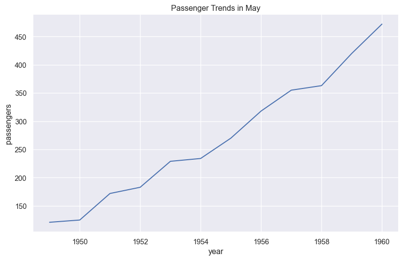
15.6 Distribution Plots
3. Histogram - Data Distribution
Histograms show the frequency distribution of a variable:
plt.figure(figsize=(10, 6))
sns.histplot(data=tips, x='total_bill', bins=20, kde=True)
plt.title('Distribution of Total Bills')
plt.xlabel('Total Bill ($)')
plt.show()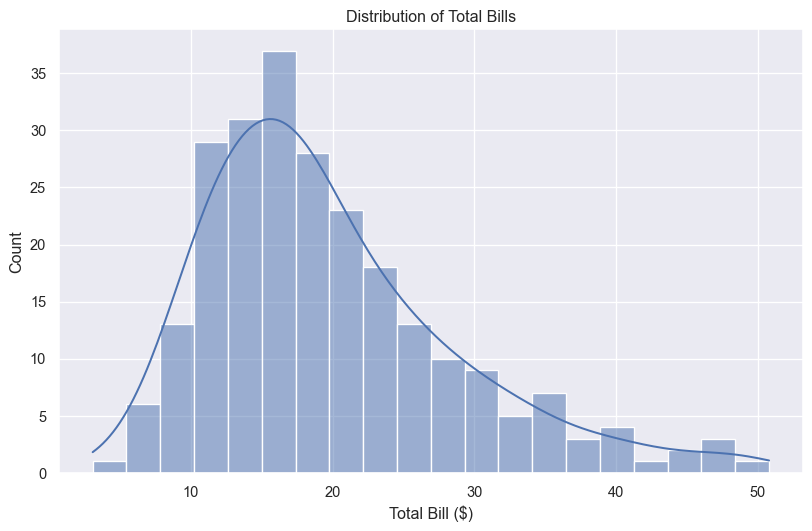
4. KDE Plot - Smooth Distribution
KDE (Kernel Density Estimation) plots show smooth probability distributions:
plt.figure(figsize=(10, 6))
sns.kdeplot(data=tips, x='total_bill', hue='time', fill=True, alpha=0.5)
plt.title('Bill Distribution by Time of Day')
plt.show()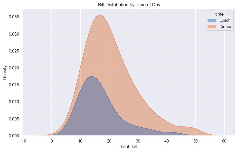
5. Box Plot - Statistical Summary
Box plots display the distribution through quartiles:
plt.figure(figsize=(10, 6))
sns.boxplot(data=tips, x='day', y='total_bill', hue='time')
plt.title('Bill Distribution by Day and Time')
plt.show()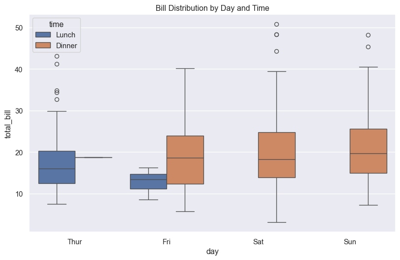
6. Violin Plot - Distribution Shape
Violin plots combine box plots with KDE:
plt.figure(figsize=(10, 6))
sns.violinplot(data=tips, x='day', y='total_bill', hue='sex', split=True)
plt.title('Bill Distribution by Day and Gender')
plt.show()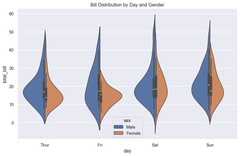
15.7 Categorical Plots
7. Bar Plot - Category Averages
Bar plots show average values for categories:
plt.figure(figsize=(10, 6))
sns.barplot(data=tips, x='day', y='total_bill', estimator=np.mean, errorbar='sd')
plt.title('Average Bill by Day')
plt.ylabel('Average Total Bill ($)')
plt.show()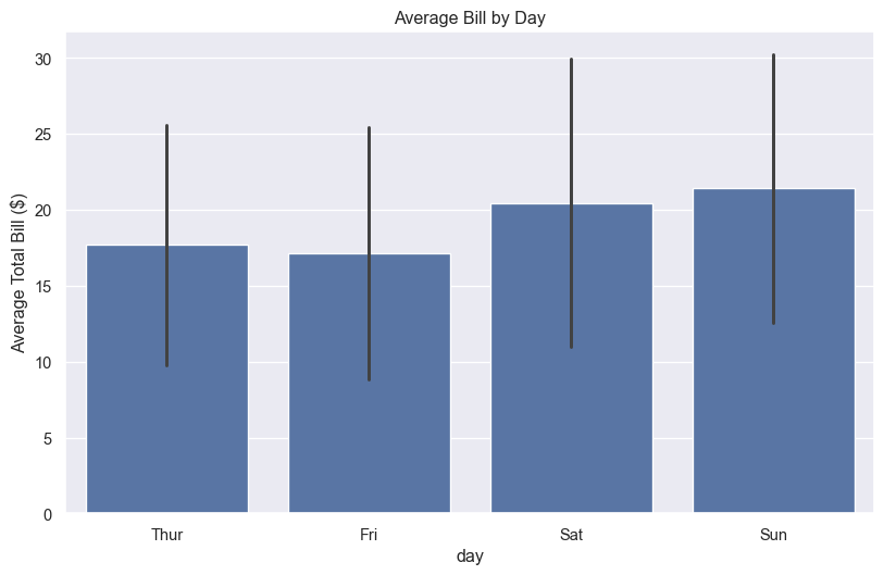
8. Count Plot - Category Frequencies
Count plots show the frequency of categorical values:
plt.figure(figsize=(10, 6))
sns.countplot(data=tips, x='day', hue='time')
plt.title('Number of Visits by Day and Time')
plt.show()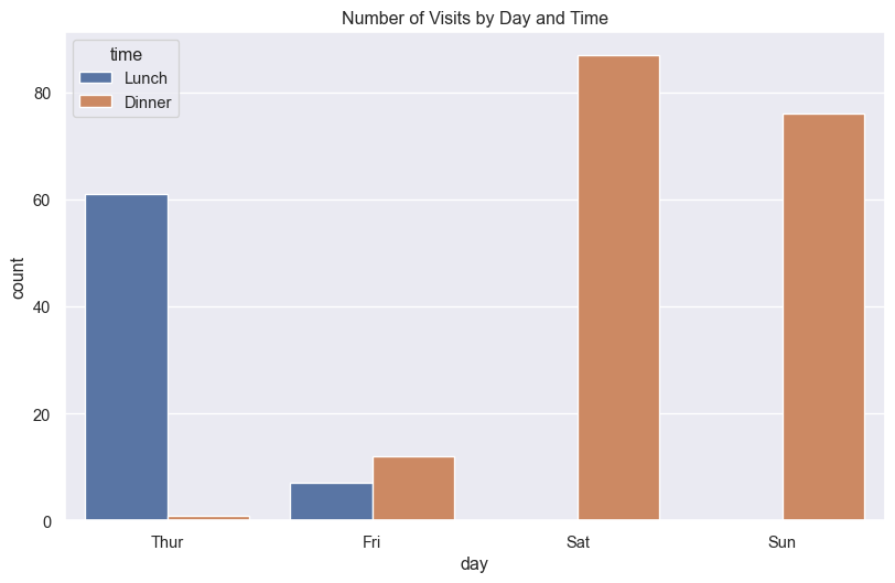
9. Strip Plot - Individual Points
Strip plots show all individual data points:
plt.figure(figsize=(10, 6))
sns.stripplot(data=tips, x='day', y='tip', hue='time', dodge=True, alpha=0.7)
plt.title('Individual Tips by Day and Time')
plt.show()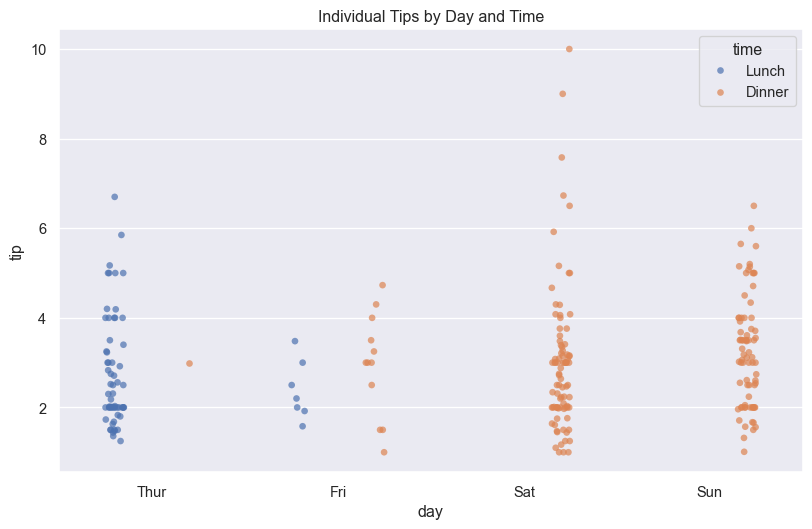
10. Swarm Plot - Non-overlapping Points
Swarm plots arrange points to avoid overlap:
plt.figure(figsize=(10, 6))
sns.swarmplot(data=tips, x='day', y='tip', hue='time', dodge=True)
plt.title('Tip Distribution (Swarm Plot)')
plt.show()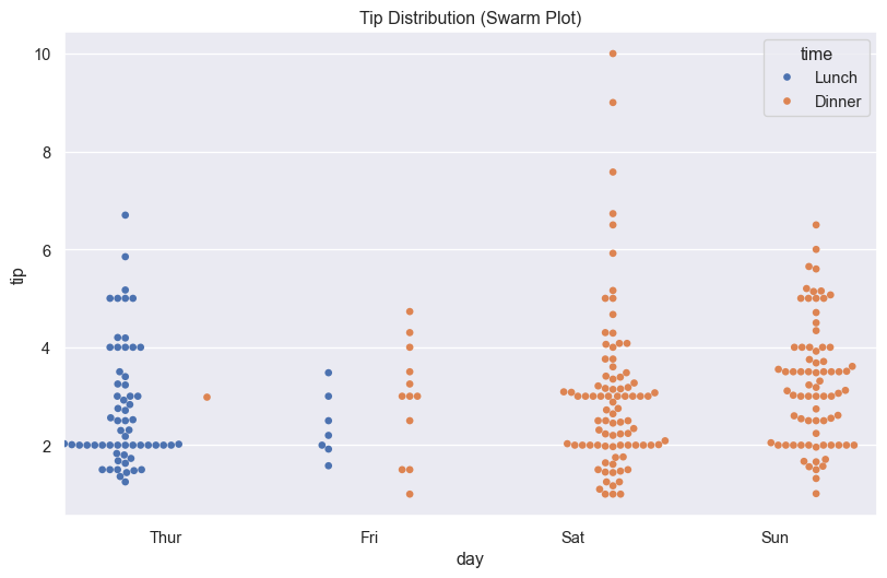
15.8 Multi-Plot Grids
11. Pair Plot - Multiple Relationships
Pair plots show relationships between all variable pairs:
# Create pair plot for numerical variables
sns.pairplot(tips, hue='time', diag_kind='kde', height=2.5)
plt.suptitle('Pair Plot of Tips Dataset', y=1.02)
plt.show()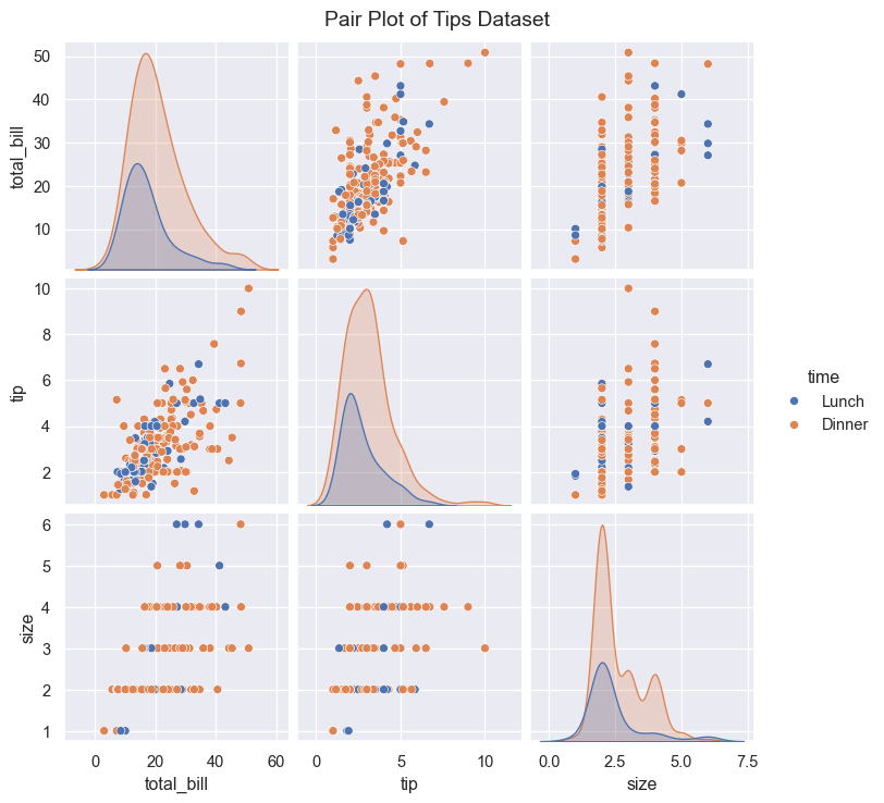
12. FacetGrid - Subplots by Category
FacetGrid creates multiple subplots based on categories:
# Create a grid of plots by time and smoker status
g = sns.FacetGrid(tips, col='time', row='smoker', height=4, aspect=1.2)
g.map(sns.scatterplot, 'total_bill', 'tip', alpha=0.7)
g.add_legend()
plt.show()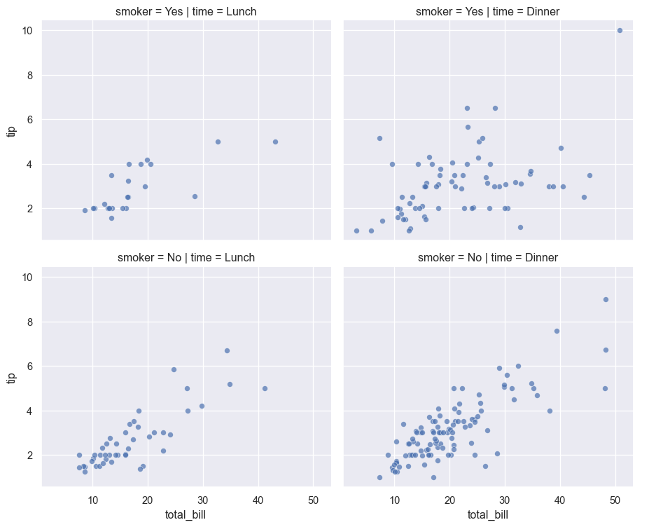
15.9 Relationship Plots
13. Regression Plot - Linear Relationships
Regression plots fit and visualize linear relationships:
plt.figure(figsize=(10, 6))
sns.regplot(data=tips, x='total_bill', y='tip', scatter_kws={'alpha':0.5})
plt.title('Linear Relationship: Bill vs Tip')
plt.show()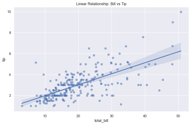
14. Joint Plot - Bivariate Distribution
Joint plots combine scatter plots with distribution plots:
sns.jointplot(data=tips, x='total_bill', y='tip', hue='time', height=8)
plt.show()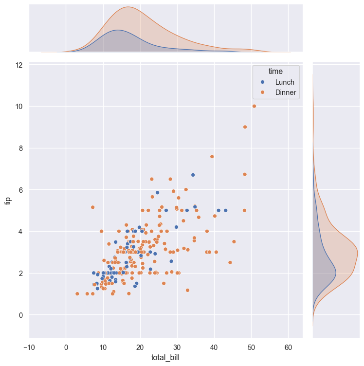
15. Heatmap - Correlation Matrix
Heatmaps visualize data matrices and correlations:
# Calculate correlation matrix
numerical_cols = tips.select_dtypes(include=[np.number])
correlation = numerical_cols.corr()

# Create heatmap
plt.figure(figsize=(8, 6))
sns.heatmap(correlation, annot=True, cmap='coolwarm', center=0,
            square=True, linewidths=1, fmt='.2f')
plt.title('Correlation Heatmap')
plt.show()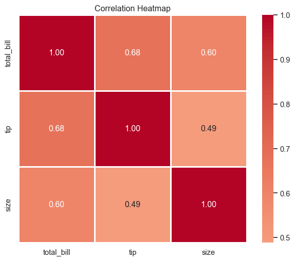
15.10 Customization and Styling
Themes and Styles
Seaborn provides several built-in themes:
# Available styles: darkgrid, whitegrid, dark, white, ticks
styles = ['darkgrid', 'whitegrid', 'dark', 'white', 'ticks']

fig, axes = plt.subplots(2, 3, figsize=(15, 8))
axes = axes.flatten()

for idx, style in enumerate(styles):
    sns.set_style(style)
    plt.sca(axes[idx])
    sns.scatterplot(data=tips, x='total_bill', y='tip', alpha=0.6)
    axes[idx].set_title(f'Style: {style}')

# Remove extra subplot
axes[-1].remove()

plt.tight_layout()
plt.show()

# Reset to default
sns.set_style('darkgrid')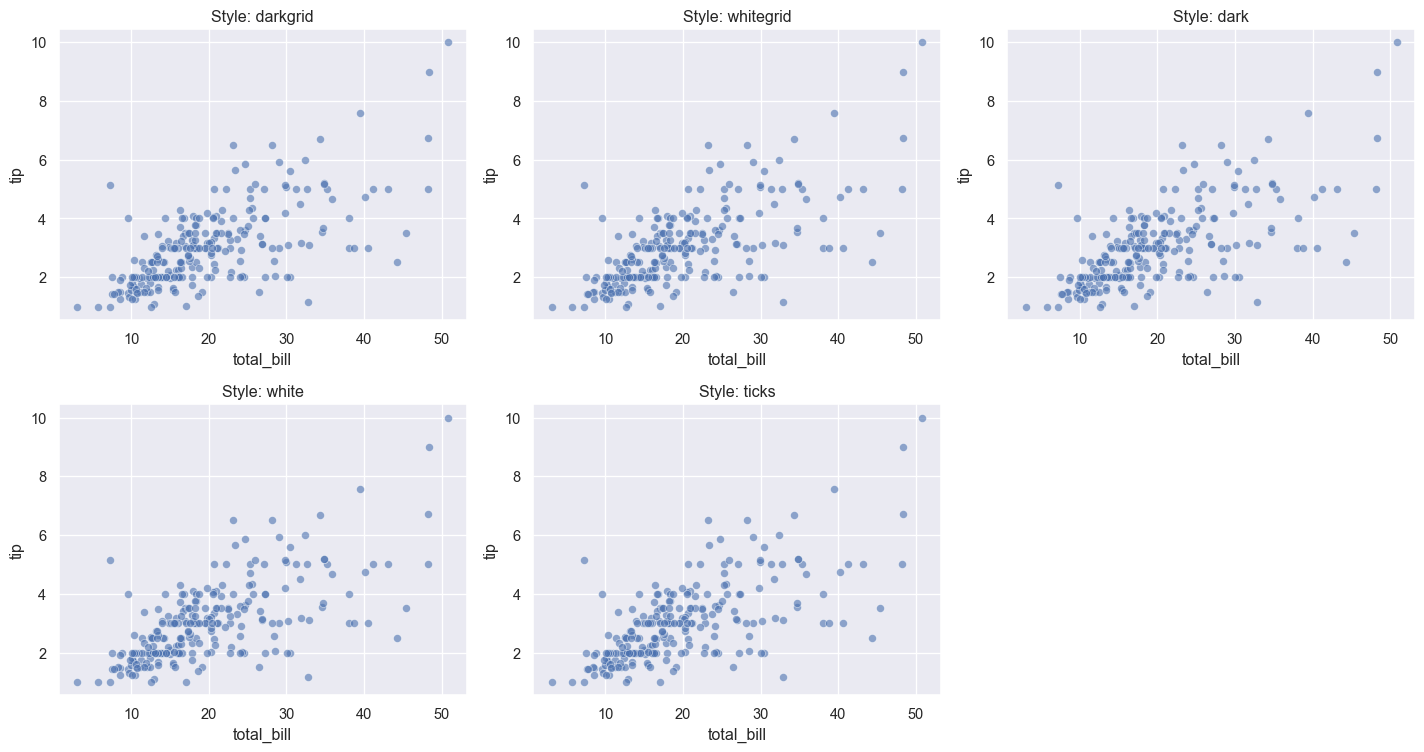
Color Palettes
Seaborn offers many color palettes:
# Show different color palettes
palettes = ['deep', 'muted', 'pastel', 'bright', 'dark', 'colorblind']

fig, axes = plt.subplots(2, 3, figsize=(15, 8))
axes = axes.flatten()

for idx, palette in enumerate(palettes):
    plt.sca(axes[idx])
    sns.barplot(data=tips, x='day', y='total_bill', palette=palette)
    axes[idx].set_title(f'Palette: {palette}')
    axes[idx].set_ylabel('')

plt.tight_layout()
plt.show()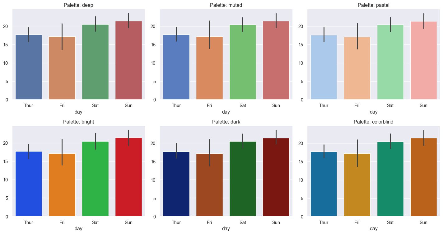
Custom Colors
# Use custom color palette
custom_colors = ['#FF6B6B', '#4ECDC4', '#45B7D1', '#FFA07A']

plt.figure(figsize=(10, 6))
sns.boxplot(data=tips, x='day', y='total_bill', palette=custom_colors)
plt.title('Custom Color Palette')
plt.show()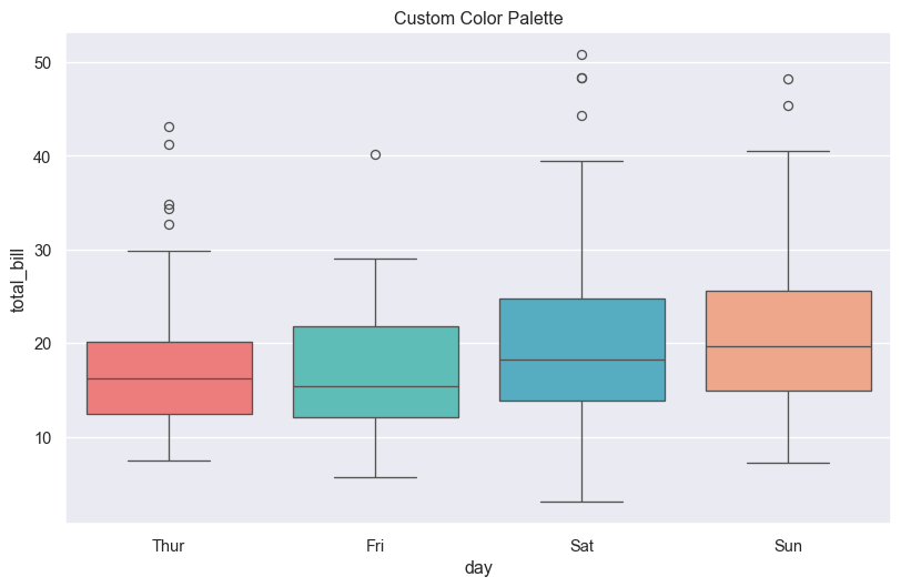
Figure Size and Context
Control the size and scale of plot elements:
# Available contexts: paper, notebook, talk, poster
contexts = ['paper', 'notebook', 'talk', 'poster']

fig, axes = plt.subplots(2, 2, figsize=(15, 12))
axes = axes.flatten()

for idx, context in enumerate(contexts):
    sns.set_context(context)
    plt.sca(axes[idx])
    sns.scatterplot(data=tips, x='total_bill', y='tip')
    axes[idx].set_title(f'Context: {context}')

plt.tight_layout()
plt.show()

# Reset to default
sns.set_context('notebook')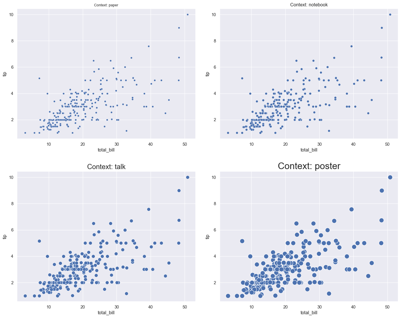
15.11 Advanced Customization
# Combine multiple customizations
plt.figure(figsize=(12, 7))

# Set style and palette
sns.set_style('whitegrid')
sns.set_palette('husl')

# Create plot
ax = sns.violinplot(data=tips, x='day', y='total_bill', hue='time')

# Customize labels and title
plt.title('Restaurant Bills by Day and Time', fontsize=16, fontweight='bold')
plt.xlabel('Day of Week', fontsize=12)
plt.ylabel('Total Bill ($)', fontsize=12)

# Customize legend
plt.legend(title='Meal Time', title_fontsize=12, fontsize=10, loc='upper right')

# Add grid
plt.grid(axis='y', alpha=0.3)

plt.tight_layout()
plt.show()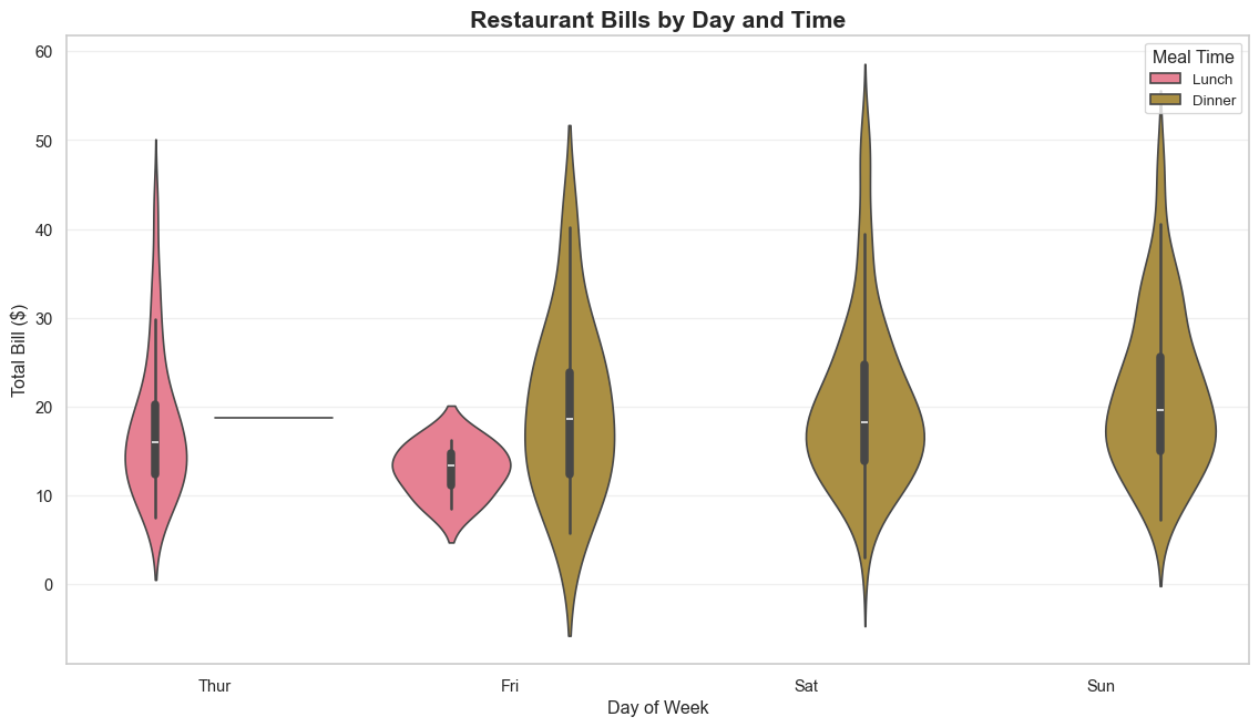
15.12 Real-World Example: Complete Analysis
Let’s put it all together with a complete analysis:
# Load iris dataset
iris = sns.load_dataset('iris')

# Create a comprehensive figure
fig = plt.figure(figsize=(16, 10))

## Pair plot for overview
plt.subplot(2, 3, 1)
# Note: pair plot creates its own figure, so we'll use other plots

## Distribution of petal length
plt.subplot(2, 3, 1)
sns.histplot(data=iris, x='petal_length', hue='species', kde=True, alpha=0.6)
plt.title('Petal Length Distribution by Species')

## Relationship between petal dimensions
plt.subplot(2, 3, 2)
sns.scatterplot(data=iris, x='petal_length', y='petal_width',
                hue='species', style='species', s=100)
plt.title('Petal Dimensions by Species')

## Box plot of sepal length
plt.subplot(2, 3, 3)
sns.boxplot(data=iris, x='species', y='sepal_length', palette='Set2')
plt.title('Sepal Length by Species')
plt.xticks(rotation=45)

## Violin plot of sepal width
plt.subplot(2, 3, 4)
sns.violinplot(data=iris, x='species', y='sepal_width', palette='Set2')
plt.title('Sepal Width Distribution')
plt.xticks(rotation=45)

## Correlation heatmap
plt.subplot(2, 3, 5)
iris_numeric = iris.select_dtypes(include=[np.number])
sns.heatmap(iris_numeric.corr(), annot=True, cmap='coolwarm',
            center=0, square=True, fmt='.2f')
plt.title('Feature Correlations')

## Count plot
plt.subplot(2, 3, 6)
sns.countplot(data=iris, x='species', palette='Set2')
plt.title('Sample Count by Species')
plt.xticks(rotation=45)

plt.suptitle('Iris Dataset: Comprehensive Analysis', fontsize=16, fontweight='bold', y=1.00)
plt.tight_layout()
plt.show()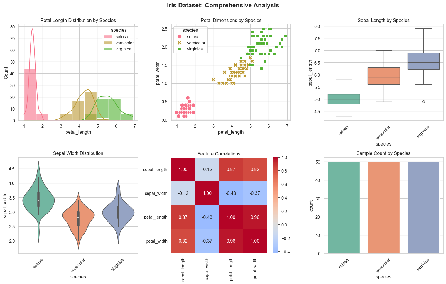
15.13 Practice Exercises
Now it’s your turn! Try these exercises:
Exercise 1: Basic Plot
Load the ‘penguins’ dataset and create a scatter plot showing the relationship between bill_length_mm and bill_depth_mm, colored by species.
# Your code here:
penguins = sns.load_dataset('penguins')
# Create your scatter plot
Exercise 2: Distribution Analysis
Using the penguins dataset, create a violin plot showing the distribution of body_mass_g for each species.
# Your code here:Exercise 3: Multi-variable Visualization
Create a FacetGrid with the tips dataset showing scatter plots of total_bill vs tip for each combination of time (columns) and sex (rows).
# Your code here:Exercise 4: Custom Styling
Create a box plot of your choice and customize it with: - A custom color palette - A specific style (e.g., ‘whitegrid’) - Custom title and labels - Rotated x-axis labels
# Your code here:15.14 Solutions
Solution 1:
Click to show solution
penguins = sns.load_dataset('penguins')

plt.figure(figsize=(10, 6))
sns.scatterplot(data=penguins, x='bill_length_mm', y='bill_depth_mm',
                hue='species', style='species', s=100)
plt.title('Penguin Bill Dimensions by Species')
plt.xlabel('Bill Length (mm)')
plt.ylabel('Bill Depth (mm)')
plt.show()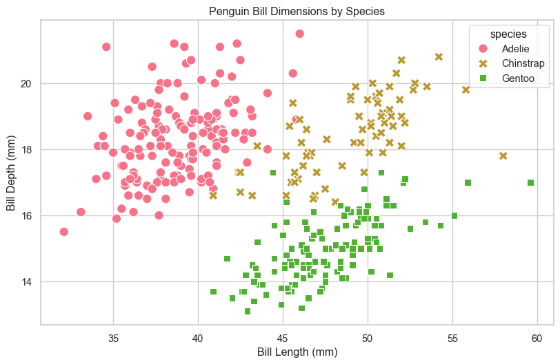
Solution 2:
Click to show solution
plt.figure(figsize=(10, 6))
sns.violinplot(data=penguins, x='species', y='body_mass_g', palette='muted')
plt.title('Penguin Body Mass Distribution by Species')
plt.xlabel('Species')
plt.ylabel('Body Mass (g)')
plt.show()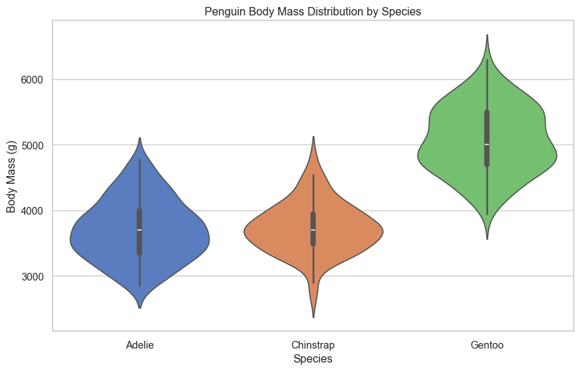
Solution 3:
Click to show solution
g = sns.FacetGrid(tips, col='time', row='sex', height=4, aspect=1.2)
g.map(sns.scatterplot, 'total_bill', 'tip', alpha=0.6)
g.add_legend()
g.fig.suptitle('Tips Analysis by Time and Gender', y=1.02)
plt.show()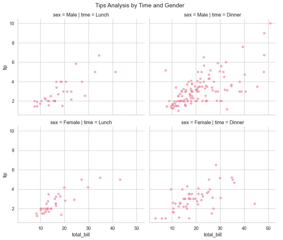
Solution 4:
Click to show solution
sns.set_style('whitegrid')

plt.figure(figsize=(12, 6))
custom_palette = ['#FF6B6B', '#4ECDC4', '#45B7D1']
sns.boxplot(data=penguins, x='island', y='flipper_length_mm',
            hue='species', palette=custom_palette)

plt.title('Penguin Flipper Length by Island and Species',
          fontsize=14, fontweight='bold')
plt.xlabel('Island', fontsize=12)
plt.ylabel('Flipper Length (mm)', fontsize=12)
plt.xticks(rotation=45)
plt.legend(title='Species', title_fontsize=11)
plt.tight_layout()
plt.show()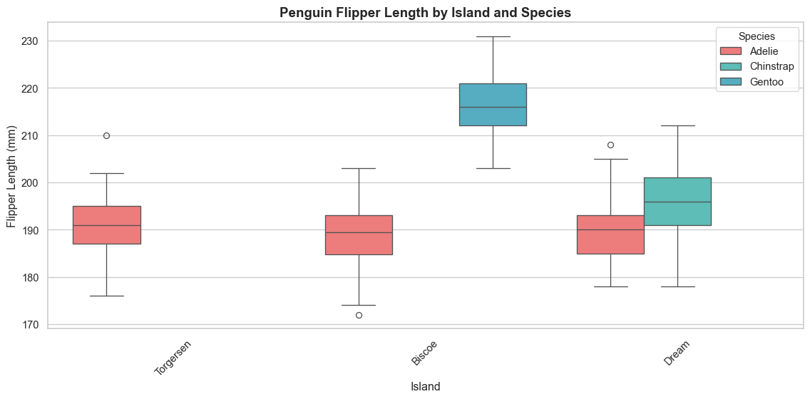
15.15 Key Takeaways
Remember:
- Import properly: Always import seaborn as
snsand matplotlib.pyplot asplt - Set themes: Use
sns.set_theme()orsns.set_style()for better-looking plots - Choose the right plot:
- Scatter/Line plots: Relationships and trends
- Histograms/KDE: Distributions
- Box/Violin plots: Statistical summaries
- Bar/Count plots: Categorical comparisons
- Heatmaps: Correlations and matrices
- Use hue and size: Add dimensions to your plots with color and size parameters
- Customize: Adjust colors, labels, and styles to make plots publication-ready
- Multi-plots: Use FacetGrid, pair plots, and joint plots for comprehensive analysis
15.16 Common Plot Types Summary
| Plot Type | Use Case | Key Parameters |
|---|---|---|
scatterplot |
Relationships between variables | x, y, hue, size |
lineplot |
Trends over time/continuous data | x, y, hue |
histplot |
Distribution of single variable | x, bins, kde |
boxplot |
Statistical summary by category | x, y, hue |
violinplot |
Distribution shape by category | x, y, hue, split |
barplot |
Average values by category | x, y, estimator |
heatmap |
Matrix data and correlations | data, annot, cmap |
pairplot |
Multiple variable relationships | data, hue |
regplot |
Linear regression | x, y |
15.17 Next Steps
Now that you understand Seaborn basics, you’re ready to: - Explore statistical estimation functions - Learn about advanced customization with matplotlib - Create interactive visualizations with Plotly - Build dashboards with Streamlit or Dash - Work with geographical data using GeoPandas
15.18 Additional Resources
- Seaborn Official Documentation: https://seaborn.pydata.org/
- Seaborn Gallery: https://seaborn.pydata.org/examples/index.html
- Color Palette Guide: https://seaborn.pydata.org/tutorial/color_palettes.html
Keep practicing and happy visualizing!