Hypothesis testing is a fundamental statistical method used to make inferences about population parameters based on sample data. It allows us to determine whether observed differences or relationships in our data are statistically significant or could have occurred by chance.
17.2 Key Concepts
Null Hypothesis (H₀): The default assumption that there is no effect or no difference.
Alternative Hypothesis (H₁ or Hₐ): The claim we’re testing for; suggests there is an effect or difference.
p-value: The probability of observing results as extreme as those in your sample, assuming the null hypothesis is true.
Significance Level (α): The threshold for rejecting the null hypothesis (commonly 0.05).
Test Statistic: A standardized value calculated from sample data used to make a decision about the hypothesis.
17.3 Parametric vs. Nonparametric Tests
Parametric tests assume that data follows a specific distribution (usually normal) and make assumptions about population parameters.
Nonparametric tests make fewer assumptions about the data distribution and are more robust to outliers and non-normal distributions.
Let’s set up our Python environment:
import numpy as npimport pandas as pdimport matplotlib.pyplot as pltimport seaborn as snsfrom scipy import statsimport warnings# Set random seed for reproducibilitynp.random.seed(42)# Configure plottingsns.set_style("whitegrid")plt.rcParams['figure.figsize'] = (10, 6)warnings.filterwarnings('ignore')print("Libraries loaded successfully!")
Libraries loaded successfully!
17.4 Parametric Tests
Parametric tests are powerful when their assumptions are met. They typically assume:
Data is normally distributed
Homogeneity of variance (for comparing groups)
Data is measured on an interval or ratio scale
Observations are independent
17.5 One-Sample t-Test
Tests whether the mean of a single sample differs from a known or hypothesized population mean.
Use case: Compare sample mean to a known value.
Assumptions: - Normal distribution - Independent observations
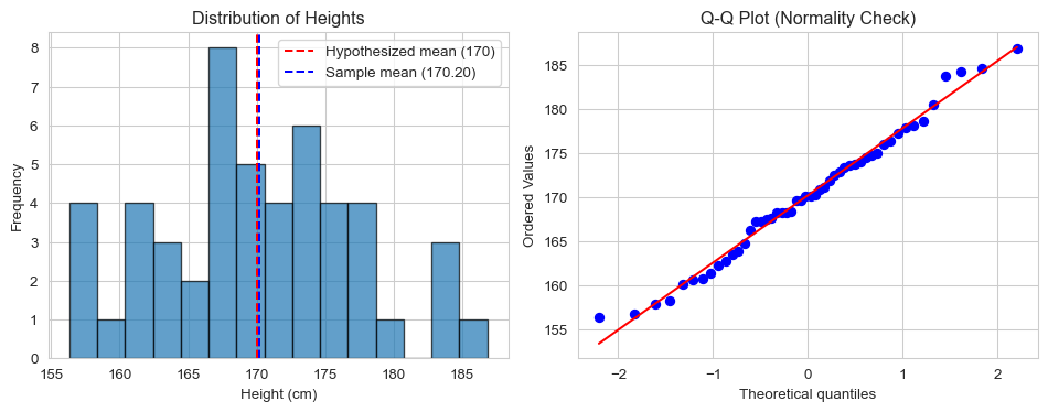
# Example: Test if average height differs from 170 cmheights = np.random.normal(loc=172, scale=8, size=50)# Visualize the dataplt.figure(figsize=(10, 4))plt.subplot(1, 2, 1)plt.hist(heights, bins=15, edgecolor='black', alpha=0.7)plt.axvline(x=170, color='red', linestyle='--', label='Hypothesized mean (170)')plt.axvline(x=np.mean(heights), color='blue', linestyle='--', label=f'Sample mean ({np.mean(heights):.2f})')plt.xlabel('Height (cm)')plt.ylabel('Frequency')plt.title('Distribution of Heights')plt.legend()plt.subplot(1, 2, 2)stats.probplot(heights, dist="norm", plot=plt)plt.title('Q-Q Plot (Normality Check)')plt.tight_layout()plt.show()# Perform one-sample t-testt_statistic, p_value = stats.ttest_1samp(heights, 170)print(f"Sample mean: {np.mean(heights):.2f}")print(f"Sample std: {np.std(heights, ddof=1):.2f}")print(f"t-statistic: {t_statistic:.4f}")print(f"p-value: {p_value:.4f}")if p_value <0.05:print("Result: Reject H₀ - The sample mean significantly differs from 170 cm")else:print("Result: Fail to reject H₀ - No significant difference from 170 cm")
Sample mean: 170.20
Sample std: 7.47
t-statistic: 0.1857
p-value: 0.8534
Result: Fail to reject H₀ - No significant difference from 170 cm
17.6 Independent Two-Sample t-Test
Tests whether the means of two independent groups differ significantly.
Use case: Compare means between two independent groups.
Assumptions: - Normal distribution in both groups - Independent observations - Equal variances (for standard t-test)
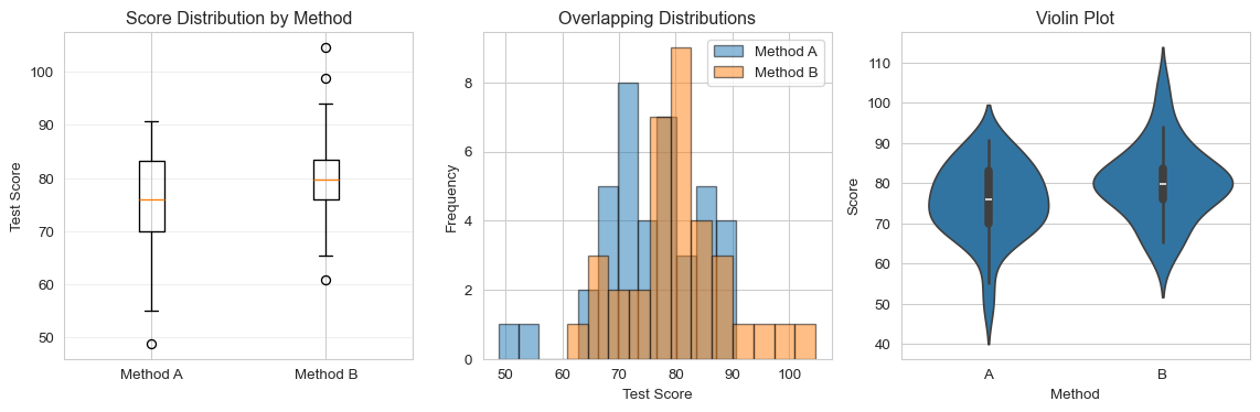
# Example: Compare test scores between two teaching methodsmethod_a = np.random.normal(loc=75, scale=10, size=40)method_b = np.random.normal(loc=80, scale=10, size=35)# Visualize the dataplt.figure(figsize=(12, 4))plt.subplot(1, 3, 1)plt.boxplot([method_a, method_b], labels=['Method A', 'Method B'])plt.ylabel('Test Score')plt.title('Score Distribution by Method')plt.grid(axis='y', alpha=0.3)plt.subplot(1, 3, 2)plt.hist(method_a, alpha=0.5, label='Method A', bins=12, edgecolor='black')plt.hist(method_b, alpha=0.5, label='Method B', bins=12, edgecolor='black')plt.xlabel('Test Score')plt.ylabel('Frequency')plt.title('Overlapping Distributions')plt.legend()plt.subplot(1, 3, 3)data_df = pd.DataFrame({'Score': np.concatenate([method_a, method_b]),'Method': ['A']*len(method_a) + ['B']*len(method_b)})sns.violinplot(x='Method', y='Score', data=data_df)plt.title('Violin Plot')plt.tight_layout()plt.show()# Check for equal variances (Levene's test)levene_stat, levene_p = stats.levene(method_a, method_b)print(f"Levene's test for equal variances: p-value = {levene_p:.4f}")# Perform independent t-test# equal_var=True for standard t-test, False for Welch's t-testt_stat, p_val = stats.ttest_ind(method_a, method_b, equal_var=(levene_p >0.05))print(f"\nMethod A - Mean: {np.mean(method_a):.2f}, Std: {np.std(method_a, ddof=1):.2f}")print(f"Method B - Mean: {np.mean(method_b):.2f}, Std: {np.std(method_b, ddof=1):.2f}")print(f"\nt-statistic: {t_stat:.4f}")print(f"p-value: {p_val:.4f}")if p_val <0.05:print("Result: Reject H₀ - Significant difference between methods")else:print("Result: Fail to reject H₀ - No significant difference")
Levene's test for equal variances: p-value = 0.7413

Method A - Mean: 75.60, Std: 9.24
Method B - Mean: 79.96, Std: 9.35

t-statistic: -2.0307
p-value: 0.0459
Result: Reject H₀ - Significant difference between methods
17.7 Paired t-Test
Tests whether the mean difference between paired observations is significantly different from zero.
Use case: Before-after measurements, matched pairs.
Assumptions: - Paired observations - Differences are normally distributed
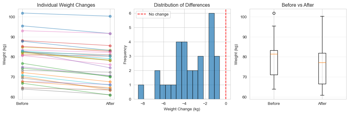
# Example: Weight before and after diet programbefore = np.random.normal(loc=80, scale=10, size=30)after = before - np.random.normal(loc=3, scale=2, size=30) # Average loss of 3 kg# Visualize paired dataplt.figure(figsize=(12, 4))plt.subplot(1, 3, 1)plt.plot([1, 2], [before, after], 'o-', alpha=0.5)plt.xticks([1, 2], ['Before', 'After'])plt.ylabel('Weight (kg)')plt.title('Individual Weight Changes')plt.grid(axis='y', alpha=0.3)plt.subplot(1, 3, 2)differences = after - beforeplt.hist(differences, bins=15, edgecolor='black', alpha=0.7)plt.axvline(x=0, color='red', linestyle='--', label='No change')plt.xlabel('Weight Change (kg)')plt.ylabel('Frequency')plt.title('Distribution of Differences')plt.legend()plt.subplot(1, 3, 3)plt.boxplot([before, after], labels=['Before', 'After'])plt.ylabel('Weight (kg)')plt.title('Before vs After')plt.grid(axis='y', alpha=0.3)plt.tight_layout()plt.show()# Perform paired t-testt_stat, p_val = stats.ttest_rel(before, after)print(f"Mean weight before: {np.mean(before):.2f} kg")print(f"Mean weight after: {np.mean(after):.2f} kg")print(f"Mean difference: {np.mean(differences):.2f} kg")print(f"\nt-statistic: {t_stat:.4f}")print(f"p-value: {p_val:.4f}")if p_val <0.05:print("Result: Reject H₀ - Significant weight change after program")else:print("Result: Fail to reject H₀ - No significant weight change")
Mean weight before: 79.04 kg
Mean weight after: 75.58 kg
Mean difference: -3.46 kg

t-statistic: 9.5454
p-value: 0.0000
Result: Reject H₀ - Significant weight change after program
17.8 One-Way ANOVA (Analysis of Variance)
Tests whether the means of three or more independent groups differ significantly.
Use case: Compare means across multiple groups.
Assumptions: - Normal distribution in each group - Independent observations - Equal variances across groups (homogeneity of variance)
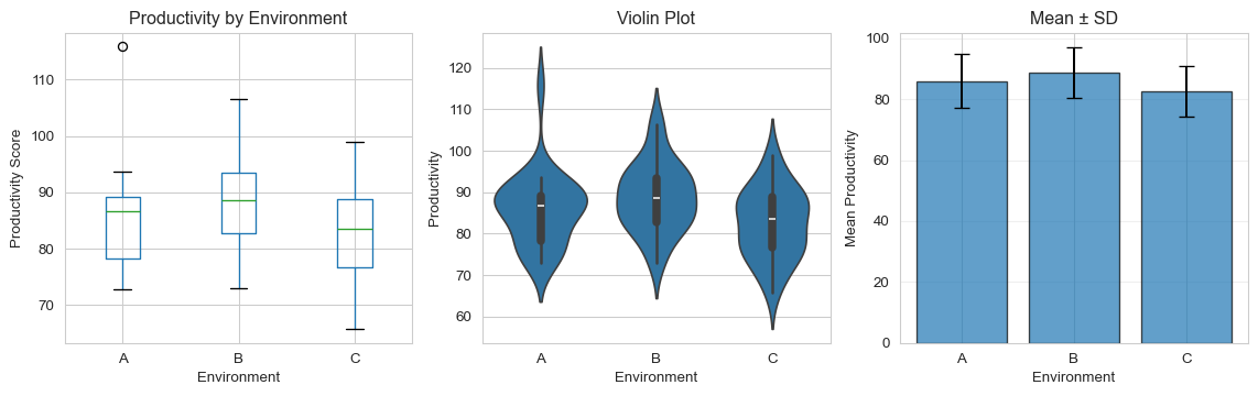
# Example: Compare productivity across three work environmentsenvironment_a = np.random.normal(loc=85, scale=8, size=25)environment_b = np.random.normal(loc=88, scale=8, size=25)environment_c = np.random.normal(loc=82, scale=8, size=25)# Create DataFrame for easier manipulationdata = pd.DataFrame({'Productivity': np.concatenate([environment_a, environment_b, environment_c]),'Environment': ['A']*25+ ['B']*25+ ['C']*25})# Visualize the dataplt.figure(figsize=(12, 4))plt.subplot(1, 3, 1)data.boxplot(column='Productivity', by='Environment', ax=plt.gca())plt.title('Productivity by Environment')plt.suptitle('')plt.ylabel('Productivity Score')plt.subplot(1, 3, 2)sns.violinplot(x='Environment', y='Productivity', data=data)plt.title('Violin Plot')plt.subplot(1, 3, 3)means = data.groupby('Environment')['Productivity'].mean()stds = data.groupby('Environment')['Productivity'].std()plt.bar(means.index, means.values, yerr=stds.values, capsize=5, alpha=0.7, edgecolor='black')plt.ylabel('Mean Productivity')plt.xlabel('Environment')plt.title('Mean ± SD')plt.grid(axis='y', alpha=0.3)plt.tight_layout()plt.show()# Check for equal variances (Levene's test)levene_stat, levene_p = stats.levene(environment_a, environment_b, environment_c)print(f"Levene's test for equal variances: p-value = {levene_p:.4f}")# Perform one-way ANOVAf_statistic, p_value = stats.f_oneway(environment_a, environment_b, environment_c)print(f"\nGroup means:")print(f"Environment A: {np.mean(environment_a):.2f}")print(f"Environment B: {np.mean(environment_b):.2f}")print(f"Environment C: {np.mean(environment_c):.2f}")print(f"\nF-statistic: {f_statistic:.4f}")print(f"p-value: {p_value:.4f}")if p_value <0.05:print("Result: Reject H₀ - At least one environment differs significantly")print("Note: Post-hoc tests needed to identify which groups differ")else:print("Result: Fail to reject H₀ - No significant differences among environments")
Levene's test for equal variances: p-value = 0.8314

Group means:
Environment A: 85.96
Environment B: 88.79
Environment C: 82.49

F-statistic: 3.4536
p-value: 0.0370
Result: Reject H₀ - At least one environment differs significantly
Note: Post-hoc tests needed to identify which groups differ
17.9 Chi-Square Test for Independence
Tests whether two categorical variables are independent.
Use case: Analyze relationships between categorical variables.
Assumptions: - Independent observations - Expected frequency in each cell ≥ 5
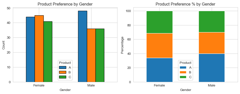
# Example: Relationship between gender and product preferencedata_categorical = pd.DataFrame({'Gender': ['Male']*120+ ['Female']*130,'Product': np.random.choice(['A', 'B', 'C'], size=250, p=[0.4, 0.35, 0.25])})# Create contingency tablecontingency_table = pd.crosstab(data_categorical['Gender'], data_categorical['Product'])print("Contingency Table:")print(contingency_table)print()# Visualizeplt.figure(figsize=(10, 4))plt.subplot(1, 2, 1)contingency_table.plot(kind='bar', ax=plt.gca(), edgecolor='black')plt.title('Product Preference by Gender')plt.xlabel('Gender')plt.ylabel('Count')plt.legend(title='Product')plt.xticks(rotation=0)plt.subplot(1, 2, 2)contingency_table_pct = contingency_table.div(contingency_table.sum(axis=1), axis=0) *100contingency_table_pct.plot(kind='bar', stacked=True, ax=plt.gca())plt.title('Product Preference % by Gender')plt.xlabel('Gender')plt.ylabel('Percentage')plt.legend(title='Product')plt.xticks(rotation=0)plt.tight_layout()plt.show()# Perform chi-square testchi2, p_value, dof, expected_freq = stats.chi2_contingency(contingency_table)print(f"Chi-square statistic: {chi2:.4f}")print(f"p-value: {p_value:.4f}")print(f"Degrees of freedom: {dof}")print("\nExpected frequencies:")print(pd.DataFrame(expected_freq, index=contingency_table.index, columns=contingency_table.columns))if p_value <0.05:print("\nResult: Reject H₀ - Gender and product preference are dependent")else:print("\nResult: Fail to reject H₀ - Gender and product preference are independent")
Contingency Table:
Product   A   B   C
Gender
Female   44  45  41
Male     48  36  36
Chi-square statistic: 1.1003
p-value: 0.5768
Degrees of freedom: 2

Expected frequencies:
Product      A      B      C
Gender
Female   47.84  42.12  40.04
Male     44.16  38.88  36.96

Result: Fail to reject H₀ - Gender and product preference are independent
17.10 Nonparametric Tests
Nonparametric tests are distribution-free and make fewer assumptions about the data. They are particularly useful when:
Data is not normally distributed
Sample size is small
Data contains outliers
Data is ordinal (ranked)
17.11 Mann-Whitney U Test (Wilcoxon Rank-Sum Test)
The nonparametric alternative to the independent two-sample t-test.
Use case: Compare two independent groups when normality cannot be assumed.
Assumptions: - Independent observations - Ordinal or continuous data
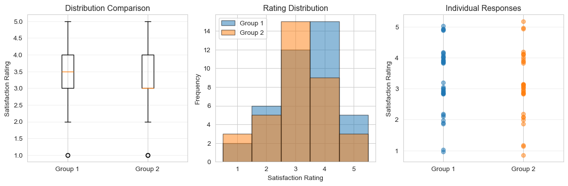
Group 1 - Median: 3.5, Mean rank: 40.55
Group 2 - Median: 3.0, Mean rank: 35.09

U-statistic: 802.0000
p-value: 0.2601
Result: Fail to reject H₀ - No significant difference
17.12 Wilcoxon Signed-Rank Test
The nonparametric alternative to the paired t-test.
Use case: Compare paired samples when normality cannot be assumed.
Assumptions: - Paired observations - Differences are symmetric around the median
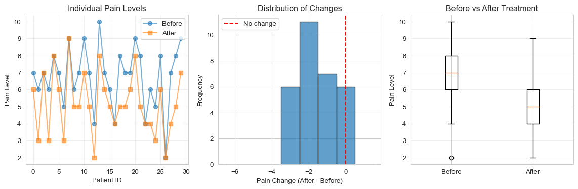
Median pain before: 7.0
Median pain after: 5.0
Median difference: -2.0

Wilcoxon statistic: 0.0000
p-value: 0.0000
Result: Reject H₀ - Significant change in pain levels
17.13 Kruskal-Wallis H Test
The nonparametric alternative to one-way ANOVA.
Use case: Compare three or more independent groups when normality cannot be assumed.
Assumptions: - Independent observations - Ordinal or continuous data
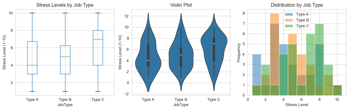
# Example: Compare stress levels across three job typesjob_type_a = np.random.choice([1, 2, 3, 4, 5, 6, 7, 8, 9, 10], size=30, p=[0.15, 0.15, 0.15, 0.15, 0.12, 0.1, 0.08, 0.05, 0.03, 0.02])job_type_b = np.random.choice([1, 2, 3, 4, 5, 6, 7, 8, 9, 10], size=28, p=[0.05, 0.08, 0.1, 0.12, 0.15, 0.15, 0.15, 0.1, 0.07, 0.03])job_type_c = np.random.choice([1, 2, 3, 4, 5, 6, 7, 8, 9, 10], size=32, p=[0.02, 0.03, 0.05, 0.08, 0.1, 0.12, 0.15, 0.17, 0.15, 0.13])# Create DataFramedata_kw = pd.DataFrame({'Stress': np.concatenate([job_type_a, job_type_b, job_type_c]),'JobType': ['Type A']*30+ ['Type B']*28+ ['Type C']*32})# Visualizeplt.figure(figsize=(12, 4))plt.subplot(1, 3, 1)data_kw.boxplot(column='Stress', by='JobType', ax=plt.gca())plt.title('Stress Levels by Job Type')plt.suptitle('')plt.ylabel('Stress Level (1-10)')plt.subplot(1, 3, 2)sns.violinplot(x='JobType', y='Stress', data=data_kw)plt.title('Violin Plot')plt.ylabel('Stress Level (1-10)')plt.subplot(1, 3, 3)for job_type in ['Type A', 'Type B', 'Type C']: job_data = data_kw[data_kw['JobType'] == job_type]['Stress'] plt.hist(job_data, alpha=0.5, label=job_type, bins=np.arange(0.5, 11.5, 1))plt.xlabel('Stress Level')plt.ylabel('Frequency')plt.title('Distribution by Job Type')plt.legend()plt.tight_layout()plt.show()# Perform Kruskal-Wallis H testh_statistic, p_value = stats.kruskal(job_type_a, job_type_b, job_type_c)print("Median stress levels:")print(f"Job Type A: {np.median(job_type_a)}")print(f"Job Type B: {np.median(job_type_b)}")print(f"Job Type C: {np.median(job_type_c)}")print(f"\nH-statistic: {h_statistic:.4f}")print(f"p-value: {p_value:.4f}")if p_value <0.05:print("Result: Reject H₀ - At least one job type has significantly different stress levels")print("Note: Post-hoc tests (e.g., pairwise Mann-Whitney) needed to identify which groups differ")else:print("Result: Fail to reject H₀ - No significant differences in stress levels")
Median stress levels:
Job Type A: 4.0
Job Type B: 5.0
Job Type C: 7.0

H-statistic: 5.4210
p-value: 0.0665
Result: Fail to reject H₀ - No significant differences in stress levels
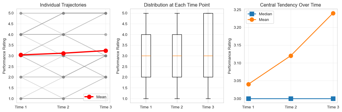
17.14 Friedman Test
The nonparametric alternative to repeated measures ANOVA.
Use case: Compare three or more related/repeated measurements.
Assumptions: - Related observations (repeated measures or matched groups) - Ordinal or continuous data
Median performance ratings:
Time 1: 3.0
Time 2: 3.0
Time 3: 3.0

Friedman statistic: 1.2400
p-value: 0.5379
Result: Fail to reject H₀ - No significant differences over time
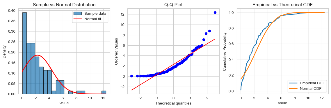
17.15 Kolmogorov-Smirnov Test
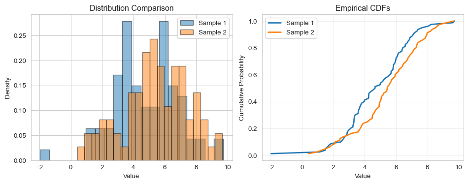
Tests whether a sample comes from a specified distribution or whether two samples come from the same distribution.
Use case: Test for normality or compare distributions.
# Example 1: Test if data follows normal distributionsample_data = np.random.exponential(scale=2, size=100)# Visualizeplt.figure(figsize=(12, 4))plt.subplot(1, 3, 1)plt.hist(sample_data, bins=20, density=True, alpha=0.7, edgecolor='black', label='Sample data')mu, sigma = np.mean(sample_data), np.std(sample_data)x = np.linspace(sample_data.min(), sample_data.max(), 100)plt.plot(x, stats.norm.pdf(x, mu, sigma), 'r-', linewidth=2, label='Normal fit')plt.xlabel('Value')plt.ylabel('Density')plt.title('Sample vs Normal Distribution')plt.legend()plt.subplot(1, 3, 2)stats.probplot(sample_data, dist="norm", plot=plt)plt.title('Q-Q Plot')plt.subplot(1, 3, 3)# Empirical CDFsorted_data = np.sort(sample_data)ecdf = np.arange(1, len(sorted_data) +1) /len(sorted_data)plt.plot(sorted_data, ecdf, label='Empirical CDF', linewidth=2)plt.plot(sorted_data, stats.norm.cdf(sorted_data, mu, sigma), label='Normal CDF', linewidth=2)plt.xlabel('Value')plt.ylabel('Cumulative Probability')plt.title('Empirical vs Theoretical CDF')plt.legend()plt.grid(alpha=0.3)plt.tight_layout()plt.show()# Test for normalityks_statistic, p_value = stats.kstest(sample_data, 'norm', args=(mu, sigma))print(f"KS statistic: {ks_statistic:.4f}")print(f"p-value: {p_value:.4f}")if p_value <0.05:print("Result: Reject H₀ - Data does not follow normal distribution")else:print("Result: Fail to reject H₀ - Data consistent with normal distribution")# Example 2: Compare two independent samplesprint("\n"+"="*60)print("Two-Sample KS Test")print("="*60)sample1 = np.random.normal(loc=5, scale=2, size=80)sample2 = np.random.normal(loc=5.5, scale=2.5, size=80)plt.figure(figsize=(10, 4))plt.subplot(1, 2, 1)plt.hist(sample1, bins=20, alpha=0.5, density=True, label='Sample 1', edgecolor='black')plt.hist(sample2, bins=20, alpha=0.5, density=True, label='Sample 2', edgecolor='black')plt.xlabel('Value')plt.ylabel('Density')plt.title('Distribution Comparison')plt.legend()plt.subplot(1, 2, 2)sorted_s1 = np.sort(sample1)sorted_s2 = np.sort(sample2)ecdf1 = np.arange(1, len(sorted_s1) +1) /len(sorted_s1)ecdf2 = np.arange(1, len(sorted_s2) +1) /len(sorted_s2)plt.plot(sorted_s1, ecdf1, label='Sample 1', linewidth=2)plt.plot(sorted_s2, ecdf2, label='Sample 2', linewidth=2)plt.xlabel('Value')plt.ylabel('Cumulative Probability')plt.title('Empirical CDFs')plt.legend()plt.grid(alpha=0.3)plt.tight_layout()plt.show()ks_stat_2sample, p_val_2sample = stats.ks_2samp(sample1, sample2)print(f"\nKS statistic: {ks_stat_2sample:.4f}")print(f"p-value: {p_val_2sample:.4f}")if p_val_2sample <0.05:print("Result: Reject H₀ - Samples come from different distributions")else:print("Result: Fail to reject H₀ - Samples likely from same distribution")
KS statistic: 0.1500
p-value: 0.0199
Result: Reject H₀ - Data does not follow normal distribution

============================================================
Two-Sample KS Test
============================================================
KS statistic: 0.2125
p-value: 0.0537
Result: Fail to reject H₀ - Samples likely from same distribution
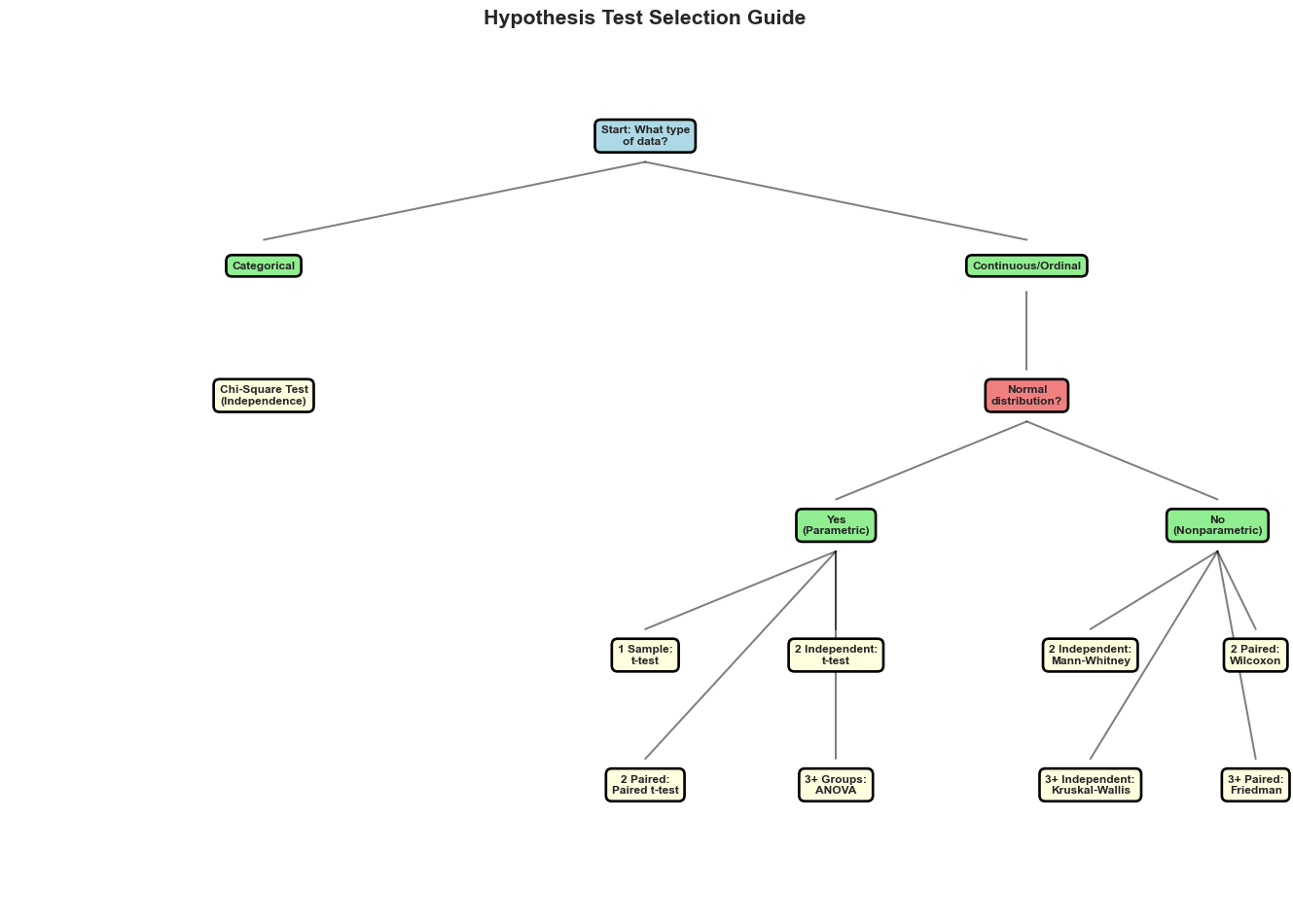
18 Choosing the Right Test
Here’s a decision guide for selecting the appropriate hypothesis test:
                Test          Type         Groups          Data Type          Assumptions
   One-Sample t-test    Parametric              1         Continuous            Normality
   Two-Sample t-test    Parametric  2 Independent         Continuous Normality, Equal var
       Paired t-test    Parametric       2 Paired         Continuous    Normality of diff
       One-Way ANOVA    Parametric 3+ Independent         Continuous Normality, Equal var
          Chi-Square    Parametric 2+ Categorical        Categorical    Expected freq ≥ 5
      Mann-Whitney U Nonparametric  2 Independent Ordinal/Continuous      Independent obs
Wilcoxon Signed-Rank Nonparametric       2 Paired Ordinal/Continuous       Symmetric diff
    Kruskal-Wallis H Nonparametric 3+ Independent Ordinal/Continuous      Independent obs
            Friedman Nonparametric      3+ Paired Ordinal/Continuous          Related obs
  Kolmogorov-Smirnov Nonparametric         1 or 2         Continuous      Continuous dist
18.3 Practical Considerations
18.4 Checking Assumptions
Before applying parametric tests, always check assumptions:
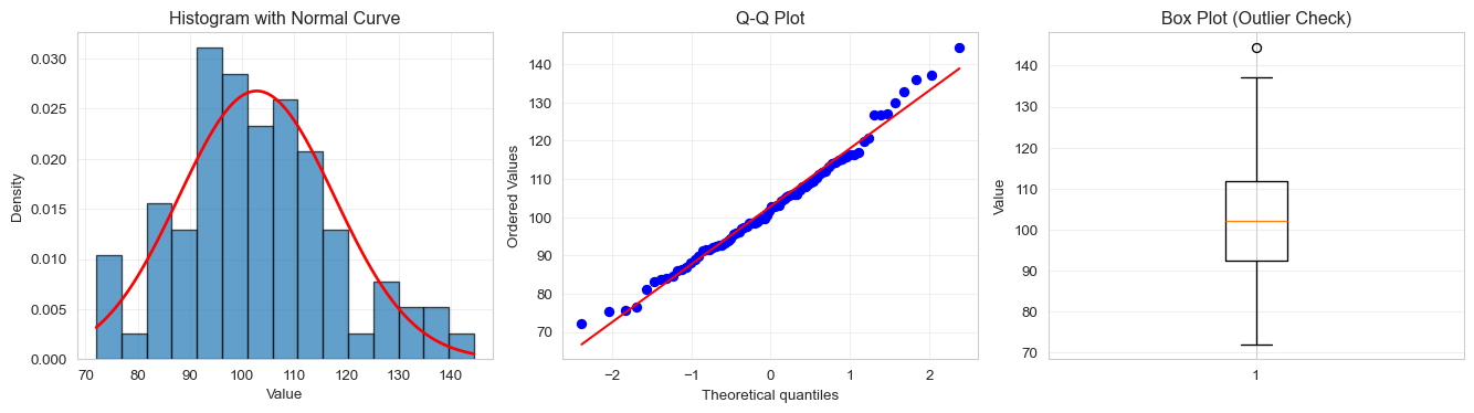
def check_parametric_assumptions(data, group_label=None):""" Comprehensive function to check parametric test assumptions """print("="*60)print("ASSUMPTION CHECKS FOR PARAMETRIC TESTS")print("="*60)# 1. Normality test (Shapiro-Wilk)print("\n1. NORMALITY TEST (Shapiro-Wilk)")print("-"*40)if group_label isNone: stat, p_value = stats.shapiro(data)print(f"Statistic: {stat:.4f}, p-value: {p_value:.4f}")if p_value >0.05:print("✓ Data appears normally distributed (p > 0.05)")else:print("✗ Data may not be normally distributed (p ≤ 0.05)")print(" Consider nonparametric alternative")# 2. Visual normality checkprint("\n2. VISUAL CHECKS")print("-"*40) fig, axes = plt.subplots(1, 3, figsize=(14, 4))# Histogram with normal curve axes[0].hist(data, bins=15, density=True, alpha=0.7, edgecolor='black') mu, sigma = np.mean(data), np.std(data) x = np.linspace(data.min(), data.max(), 100) axes[0].plot(x, stats.norm.pdf(x, mu, sigma), 'r-', linewidth=2) axes[0].set_xlabel('Value') axes[0].set_ylabel('Density') axes[0].set_title('Histogram with Normal Curve') axes[0].grid(alpha=0.3)# Q-Q plot stats.probplot(data, dist="norm", plot=axes[1]) axes[1].set_title('Q-Q Plot') axes[1].grid(alpha=0.3)# Box plot axes[2].boxplot(data) axes[2].set_ylabel('Value') axes[2].set_title('Box Plot (Outlier Check)') axes[2].grid(axis='y', alpha=0.3) plt.tight_layout() plt.show()# 3. Outlier detectionprint("\n3. OUTLIER DETECTION")print("-"*40) Q1 = np.percentile(data, 25) Q3 = np.percentile(data, 75) IQR = Q3 - Q1 outliers = data[(data < Q1 -1.5*IQR) | (data > Q3 +1.5*IQR)]print(f"IQR: {IQR:.2f}")print(f"Number of outliers: {len(outliers)}")iflen(outliers) >0:print(f"Outlier values: {outliers[:10]}") # Show first 10print("⚠ Consider impact of outliers or use robust methods")else:print("✓ No outliers detected")# 4. Descriptive statisticsprint("\n4. DESCRIPTIVE STATISTICS")print("-"*40)print(f"Mean: {np.mean(data):.2f}")print(f"Median: {np.median(data):.2f}")print(f"Std Dev: {np.std(data, ddof=1):.2f}")print(f"Skewness: {stats.skew(data):.2f}")print(f"Kurtosis: {stats.kurtosis(data):.2f}")print("\n"+"="*60)# Example usagesample = np.random.normal(loc=100, scale=15, size=80)check_parametric_assumptions(sample)
============================================================
ASSUMPTION CHECKS FOR PARAMETRIC TESTS
============================================================

1. NORMALITY TEST (Shapiro-Wilk)
----------------------------------------
Statistic: 0.9840, p-value: 0.4206
✓ Data appears normally distributed (p > 0.05)

2. VISUAL CHECKS
----------------------------------------
3. OUTLIER DETECTION
----------------------------------------
IQR: 19.21
Number of outliers: 1
Outlier values: [144.47515528]
⚠ Consider impact of outliers or use robust methods

4. DESCRIPTIVE STATISTICS
----------------------------------------
Mean: 102.82
Median: 102.20
Std Dev: 15.00
Skewness: 0.41
Kurtosis: 0.07

============================================================
18.5 Effect Size and Power
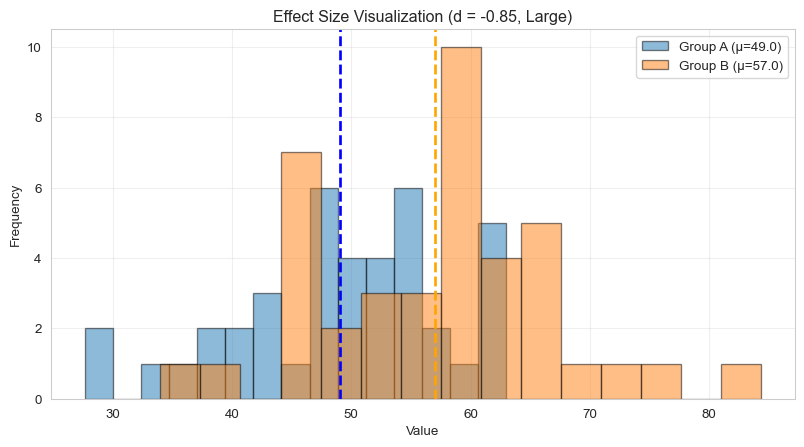
Statistical significance (p-value) doesn’t tell the whole story. Effect size measures the magnitude of differences:
def cohens_d(group1, group2):""" Calculate Cohen's d for effect size between two groups Interpretation: - Small effect: d = 0.2 - Medium effect: d = 0.5 - Large effect: d = 0.8 """ n1, n2 =len(group1), len(group2) var1, var2 = np.var(group1, ddof=1), np.var(group2, ddof=1) pooled_std = np.sqrt(((n1-1)*var1 + (n2-1)*var2) / (n1+n2-2))return (np.mean(group1) - np.mean(group2)) / pooled_std# Examplegroup_a = np.random.normal(loc=50, scale=10, size=40)group_b = np.random.normal(loc=55, scale=10, size=40)t_stat, p_val = stats.ttest_ind(group_a, group_b)effect_size = cohens_d(group_a, group_b)print("Effect Size Analysis")print("="*60)print(f"Group A mean: {np.mean(group_a):.2f}")print(f"Group B mean: {np.mean(group_b):.2f}")print(f"Difference: {np.mean(group_b) - np.mean(group_a):.2f}")print(f"\nt-statistic: {t_stat:.4f}")print(f"p-value: {p_val:.4f}")print(f"\nCohen's d: {effect_size:.4f}")ifabs(effect_size) <0.2: effect_interpretation ="Negligible"elifabs(effect_size) <0.5: effect_interpretation ="Small"elifabs(effect_size) <0.8: effect_interpretation ="Medium"else: effect_interpretation ="Large"print(f"Effect size interpretation: {effect_interpretation}")# Visualizeplt.figure(figsize=(10, 5))plt.hist(group_a, bins=15, alpha=0.5, label=f'Group A (μ={np.mean(group_a):.1f})', edgecolor='black')plt.hist(group_b, bins=15, alpha=0.5, label=f'Group B (μ={np.mean(group_b):.1f})', edgecolor='black')plt.axvline(np.mean(group_a), color='blue', linestyle='--', linewidth=2)plt.axvline(np.mean(group_b), color='orange', linestyle='--', linewidth=2)plt.xlabel('Value')plt.ylabel('Frequency')plt.title(f'Effect Size Visualization (d = {effect_size:.2f}, {effect_interpretation})')plt.legend()plt.grid(alpha=0.3)plt.show()
Effect Size Analysis
============================================================
Group A mean: 49.04
Group B mean: 57.04
Difference: 8.00

t-statistic: -3.7861
p-value: 0.0003

Cohen's d: -0.8466
Effect size interpretation: Large
18.6 Multiple Testing Correction
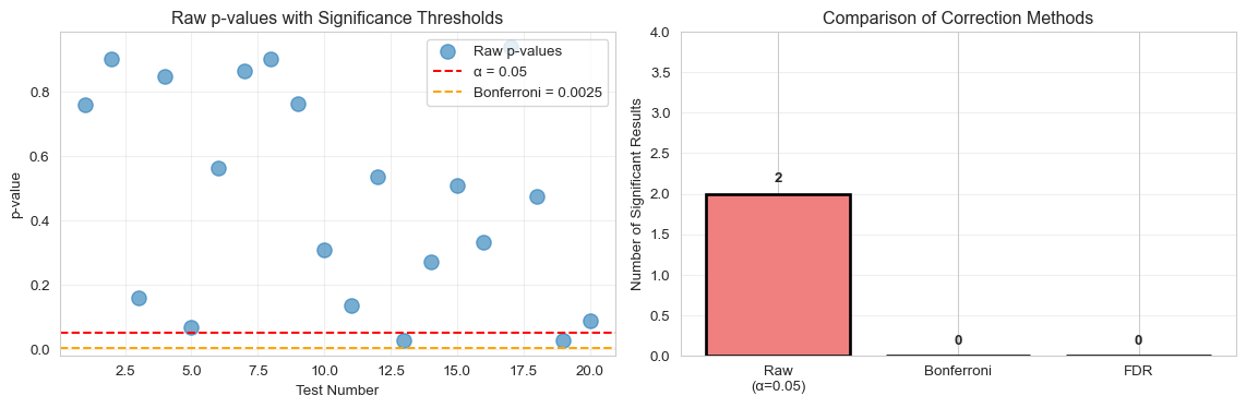
When performing multiple hypothesis tests, the probability of Type I error (false positive) increases. Apply corrections:
from statsmodels.stats.multitest import multipletests# Simulate multiple comparisonsnp.random.seed(123)n_tests =20p_values = []print("Multiple Testing Example")print("="*60)print(f"Performing {n_tests} independent t-tests...\n")for i inrange(n_tests):# Most from same distribution (null is true)if i <18: group1 = np.random.normal(loc=50, scale=10, size=30) group2 = np.random.normal(loc=50, scale=10, size=30)else: # Two genuinely different group1 = np.random.normal(loc=50, scale=10, size=30) group2 = np.random.normal(loc=58, scale=10, size=30) _, p_val = stats.ttest_ind(group1, group2) p_values.append(p_val)p_values = np.array(p_values)# Apply correctionsreject_none, pvals_bonf, _, _ = multipletests(p_values, method='bonferroni')reject_fdr, pvals_fdr, _, _ = multipletests(p_values, method='fdr_bh')# Create comparison DataFrameresults_df = pd.DataFrame({'Test': range(1, n_tests +1),'Raw p-value': p_values,'Bonferroni p': pvals_bonf,'FDR p': pvals_fdr,'Raw Sig': p_values <0.05,'Bonf Sig': reject_none,'FDR Sig': reject_fdr})print(results_df.to_string(index=False))print("\n"+"="*60)print("SUMMARY")print("="*60)print(f"Significant with raw p < 0.05: {np.sum(p_values <0.05)}")print(f"Significant with Bonferroni: {np.sum(reject_none)}")print(f"Significant with FDR: {np.sum(reject_fdr)}")# Visualizeplt.figure(figsize=(12, 4))plt.subplot(1, 2, 1)x =range(1, n_tests +1)plt.scatter(x, p_values, s=100, alpha=0.6, label='Raw p-values')plt.axhline(y=0.05, color='r', linestyle='--', label='α = 0.05')plt.axhline(y=0.05/n_tests, color='orange', linestyle='--', label=f'Bonferroni = {0.05/n_tests:.4f}')plt.xlabel('Test Number')plt.ylabel('p-value')plt.title('Raw p-values with Significance Thresholds')plt.legend()plt.grid(alpha=0.3)plt.subplot(1, 2, 2)methods = ['Raw\n(α=0.05)', 'Bonferroni', 'FDR']counts = [np.sum(p_values <0.05), np.sum(reject_none), np.sum(reject_fdr)]colors = ['lightcoral', 'lightblue', 'lightgreen']bars = plt.bar(methods, counts, color=colors, edgecolor='black', linewidth=2)plt.ylabel('Number of Significant Results')plt.title('Comparison of Correction Methods')plt.ylim(0, max(counts) +2)for bar, count inzip(bars, counts): plt.text(bar.get_x() + bar.get_width()/2, bar.get_height() +0.1,str(count), ha='center', va='bottom', fontweight='bold')plt.grid(axis='y', alpha=0.3)plt.tight_layout()plt.show()
# Create a quick reference guidereference_guide = pd.DataFrame({'Situation': ['Compare sample mean to known value','Compare two independent groups (normal)','Compare two independent groups (non-normal)','Compare paired samples (normal)','Compare paired samples (non-normal)','Compare 3+ independent groups (normal)','Compare 3+ independent groups (non-normal)','Compare 3+ paired samples (non-normal)','Test independence of categorical variables','Test if sample follows specific distribution' ],'Recommended Test': ['One-sample t-test','Independent t-test','Mann-Whitney U test','Paired t-test','Wilcoxon signed-rank test','One-way ANOVA','Kruskal-Wallis H test','Friedman test','Chi-square test','Kolmogorov-Smirnov test' ],'Python Function': ['stats.ttest_1samp()','stats.ttest_ind()','stats.mannwhitneyu()','stats.ttest_rel()','stats.wilcoxon()','stats.f_oneway()','stats.kruskal()','stats.friedmanchisquare()','stats.chi2_contingency()','stats.kstest() or stats.ks_2samp()' ]})print("\n"+"="*80)print("HYPOTHESIS TESTING QUICK REFERENCE GUIDE")print("="*80+"\n")print(reference_guide.to_string(index=False))
================================================================================
HYPOTHESIS TESTING QUICK REFERENCE GUIDE
================================================================================

                                   Situation          Recommended Test                    Python Function
          Compare sample mean to known value         One-sample t-test                stats.ttest_1samp()
     Compare two independent groups (normal)        Independent t-test                  stats.ttest_ind()
 Compare two independent groups (non-normal)       Mann-Whitney U test               stats.mannwhitneyu()
             Compare paired samples (normal)             Paired t-test                  stats.ttest_rel()
         Compare paired samples (non-normal) Wilcoxon signed-rank test                   stats.wilcoxon()
      Compare 3+ independent groups (normal)             One-way ANOVA                   stats.f_oneway()
  Compare 3+ independent groups (non-normal)     Kruskal-Wallis H test                    stats.kruskal()
      Compare 3+ paired samples (non-normal)             Friedman test          stats.friedmanchisquare()
  Test independence of categorical variables           Chi-square test           stats.chi2_contingency()
Test if sample follows specific distribution   Kolmogorov-Smirnov test stats.kstest() or stats.ks_2samp()
Misinterpreting p-values: P-value is NOT the probability that H₀ is true
Conclusion: Hypothesis testing is a powerful tool for statistical inference. By understanding the assumptions, choosing appropriate tests, and interpreting results carefully, you can make sound statistical decisions in your data analysis projects.
Source Code
---title: "Inferential Statistics and Hypothesis Testing"jupyter: python3execute: eval: true echo: true warning: false---## Introduction to Hypothesis TestingHypothesis testing is a fundamental statistical method used to make inferences about population parameters based on sample data. It allows us to determine whether observed differences or relationships in our data are statistically significant or could have occurred by chance.## Key Concepts**Null Hypothesis (H₀)**: The default assumption that there is no effect or no difference.**Alternative Hypothesis (H₁ or Hₐ)**: The claim we're testing for; suggests there is an effect or difference.**p-value**: The probability of observing results as extreme as those in your sample, assuming the null hypothesis is true.**Significance Level (α)**: The threshold for rejecting the null hypothesis (commonly 0.05).**Test Statistic**: A standardized value calculated from sample data used to make a decision about the hypothesis.## Parametric vs. Nonparametric Tests**Parametric tests** assume that data follows a specific distribution (usually normal) and make assumptions about population parameters.**Nonparametric tests** make fewer assumptions about the data distribution and are more robust to outliers and non-normal distributions.Let's set up our Python environment:```{python}import numpy as npimport pandas as pdimport matplotlib.pyplot as pltimport seaborn as snsfrom scipy import statsimport warnings# Set random seed for reproducibilitynp.random.seed(42)# Configure plottingsns.set_style("whitegrid")plt.rcParams['figure.figsize'] = (10, 6)warnings.filterwarnings('ignore')print("Libraries loaded successfully!")```## Parametric TestsParametric tests are powerful when their assumptions are met. They typically assume:1. Data is normally distributed2. Homogeneity of variance (for comparing groups)3. Data is measured on an interval or ratio scale4. Observations are independent## One-Sample t-TestTests whether the mean of a single sample differs from a known or hypothesized population mean.**Use case**: Compare sample mean to a known value.**Assumptions**:- Normal distribution- Independent observations```{python}# Example: Test if average height differs from 170 cmheights = np.random.normal(loc=172, scale=8, size=50)# Visualize the dataplt.figure(figsize=(10, 4))plt.subplot(1, 2, 1)plt.hist(heights, bins=15, edgecolor='black', alpha=0.7)plt.axvline(x=170, color='red', linestyle='--', label='Hypothesized mean (170)')plt.axvline(x=np.mean(heights), color='blue', linestyle='--', label=f'Sample mean ({np.mean(heights):.2f})')plt.xlabel('Height (cm)')plt.ylabel('Frequency')plt.title('Distribution of Heights')plt.legend()plt.subplot(1, 2, 2)stats.probplot(heights, dist="norm", plot=plt)plt.title('Q-Q Plot (Normality Check)')plt.tight_layout()plt.show()# Perform one-sample t-testt_statistic, p_value = stats.ttest_1samp(heights, 170)print(f"Sample mean: {np.mean(heights):.2f}")print(f"Sample std: {np.std(heights, ddof=1):.2f}")print(f"t-statistic: {t_statistic:.4f}")print(f"p-value: {p_value:.4f}")if p_value <0.05:print("Result: Reject H₀ - The sample mean significantly differs from 170 cm")else:print("Result: Fail to reject H₀ - No significant difference from 170 cm")```## Independent Two-Sample t-TestTests whether the means of two independent groups differ significantly.**Use case**: Compare means between two independent groups.**Assumptions**:- Normal distribution in both groups- Independent observations- Equal variances (for standard t-test)```{python}# Example: Compare test scores between two teaching methodsmethod_a = np.random.normal(loc=75, scale=10, size=40)method_b = np.random.normal(loc=80, scale=10, size=35)# Visualize the dataplt.figure(figsize=(12, 4))plt.subplot(1, 3, 1)plt.boxplot([method_a, method_b], labels=['Method A', 'Method B'])plt.ylabel('Test Score')plt.title('Score Distribution by Method')plt.grid(axis='y', alpha=0.3)plt.subplot(1, 3, 2)plt.hist(method_a, alpha=0.5, label='Method A', bins=12, edgecolor='black')plt.hist(method_b, alpha=0.5, label='Method B', bins=12, edgecolor='black')plt.xlabel('Test Score')plt.ylabel('Frequency')plt.title('Overlapping Distributions')plt.legend()plt.subplot(1, 3, 3)data_df = pd.DataFrame({'Score': np.concatenate([method_a, method_b]),'Method': ['A']*len(method_a) + ['B']*len(method_b)})sns.violinplot(x='Method', y='Score', data=data_df)plt.title('Violin Plot')plt.tight_layout()plt.show()# Check for equal variances (Levene's test)levene_stat, levene_p = stats.levene(method_a, method_b)print(f"Levene's test for equal variances: p-value = {levene_p:.4f}")# Perform independent t-test# equal_var=True for standard t-test, False for Welch's t-testt_stat, p_val = stats.ttest_ind(method_a, method_b, equal_var=(levene_p >0.05))print(f"\nMethod A - Mean: {np.mean(method_a):.2f}, Std: {np.std(method_a, ddof=1):.2f}")print(f"Method B - Mean: {np.mean(method_b):.2f}, Std: {np.std(method_b, ddof=1):.2f}")print(f"\nt-statistic: {t_stat:.4f}")print(f"p-value: {p_val:.4f}")if p_val <0.05:print("Result: Reject H₀ - Significant difference between methods")else:print("Result: Fail to reject H₀ - No significant difference")```## Paired t-TestTests whether the mean difference between paired observations is significantly different from zero.**Use case**: Before-after measurements, matched pairs.**Assumptions**:- Paired observations- Differences are normally distributed```{python}# Example: Weight before and after diet programbefore = np.random.normal(loc=80, scale=10, size=30)after = before - np.random.normal(loc=3, scale=2, size=30) # Average loss of 3 kg# Visualize paired dataplt.figure(figsize=(12, 4))plt.subplot(1, 3, 1)plt.plot([1, 2], [before, after], 'o-', alpha=0.5)plt.xticks([1, 2], ['Before', 'After'])plt.ylabel('Weight (kg)')plt.title('Individual Weight Changes')plt.grid(axis='y', alpha=0.3)plt.subplot(1, 3, 2)differences = after - beforeplt.hist(differences, bins=15, edgecolor='black', alpha=0.7)plt.axvline(x=0, color='red', linestyle='--', label='No change')plt.xlabel('Weight Change (kg)')plt.ylabel('Frequency')plt.title('Distribution of Differences')plt.legend()plt.subplot(1, 3, 3)plt.boxplot([before, after], labels=['Before', 'After'])plt.ylabel('Weight (kg)')plt.title('Before vs After')plt.grid(axis='y', alpha=0.3)plt.tight_layout()plt.show()# Perform paired t-testt_stat, p_val = stats.ttest_rel(before, after)print(f"Mean weight before: {np.mean(before):.2f} kg")print(f"Mean weight after: {np.mean(after):.2f} kg")print(f"Mean difference: {np.mean(differences):.2f} kg")print(f"\nt-statistic: {t_stat:.4f}")print(f"p-value: {p_val:.4f}")if p_val <0.05:print("Result: Reject H₀ - Significant weight change after program")else:print("Result: Fail to reject H₀ - No significant weight change")```## One-Way ANOVA (Analysis of Variance)Tests whether the means of three or more independent groups differ significantly.**Use case**: Compare means across multiple groups.**Assumptions**:- Normal distribution in each group- Independent observations- Equal variances across groups (homogeneity of variance)```{python}# Example: Compare productivity across three work environmentsenvironment_a = np.random.normal(loc=85, scale=8, size=25)environment_b = np.random.normal(loc=88, scale=8, size=25)environment_c = np.random.normal(loc=82, scale=8, size=25)# Create DataFrame for easier manipulationdata = pd.DataFrame({'Productivity': np.concatenate([environment_a, environment_b, environment_c]),'Environment': ['A']*25+ ['B']*25+ ['C']*25})# Visualize the dataplt.figure(figsize=(12, 4))plt.subplot(1, 3, 1)data.boxplot(column='Productivity', by='Environment', ax=plt.gca())plt.title('Productivity by Environment')plt.suptitle('')plt.ylabel('Productivity Score')plt.subplot(1, 3, 2)sns.violinplot(x='Environment', y='Productivity', data=data)plt.title('Violin Plot')plt.subplot(1, 3, 3)means = data.groupby('Environment')['Productivity'].mean()stds = data.groupby('Environment')['Productivity'].std()plt.bar(means.index, means.values, yerr=stds.values, capsize=5, alpha=0.7, edgecolor='black')plt.ylabel('Mean Productivity')plt.xlabel('Environment')plt.title('Mean ± SD')plt.grid(axis='y', alpha=0.3)plt.tight_layout()plt.show()# Check for equal variances (Levene's test)levene_stat, levene_p = stats.levene(environment_a, environment_b, environment_c)print(f"Levene's test for equal variances: p-value = {levene_p:.4f}")# Perform one-way ANOVAf_statistic, p_value = stats.f_oneway(environment_a, environment_b, environment_c)print(f"\nGroup means:")print(f"Environment A: {np.mean(environment_a):.2f}")print(f"Environment B: {np.mean(environment_b):.2f}")print(f"Environment C: {np.mean(environment_c):.2f}")print(f"\nF-statistic: {f_statistic:.4f}")print(f"p-value: {p_value:.4f}")if p_value <0.05:print("Result: Reject H₀ - At least one environment differs significantly")print("Note: Post-hoc tests needed to identify which groups differ")else:print("Result: Fail to reject H₀ - No significant differences among environments")```## Chi-Square Test for IndependenceTests whether two categorical variables are independent.**Use case**: Analyze relationships between categorical variables.**Assumptions**:- Independent observations- Expected frequency in each cell ≥ 5```{python}# Example: Relationship between gender and product preferencedata_categorical = pd.DataFrame({'Gender': ['Male']*120+ ['Female']*130,'Product': np.random.choice(['A', 'B', 'C'], size=250, p=[0.4, 0.35, 0.25])})# Create contingency tablecontingency_table = pd.crosstab(data_categorical['Gender'], data_categorical['Product'])print("Contingency Table:")print(contingency_table)print()# Visualizeplt.figure(figsize=(10, 4))plt.subplot(1, 2, 1)contingency_table.plot(kind='bar', ax=plt.gca(), edgecolor='black')plt.title('Product Preference by Gender')plt.xlabel('Gender')plt.ylabel('Count')plt.legend(title='Product')plt.xticks(rotation=0)plt.subplot(1, 2, 2)contingency_table_pct = contingency_table.div(contingency_table.sum(axis=1), axis=0) *100contingency_table_pct.plot(kind='bar', stacked=True, ax=plt.gca())plt.title('Product Preference % by Gender')plt.xlabel('Gender')plt.ylabel('Percentage')plt.legend(title='Product')plt.xticks(rotation=0)plt.tight_layout()plt.show()# Perform chi-square testchi2, p_value, dof, expected_freq = stats.chi2_contingency(contingency_table)print(f"Chi-square statistic: {chi2:.4f}")print(f"p-value: {p_value:.4f}")print(f"Degrees of freedom: {dof}")print("\nExpected frequencies:")print(pd.DataFrame(expected_freq, index=contingency_table.index, columns=contingency_table.columns))if p_value <0.05:print("\nResult: Reject H₀ - Gender and product preference are dependent")else:print("\nResult: Fail to reject H₀ - Gender and product preference are independent")```## Nonparametric TestsNonparametric tests are distribution-free and make fewer assumptions about the data. They are particularly useful when:- Data is not normally distributed- Sample size is small- Data contains outliers- Data is ordinal (ranked)## Mann-Whitney U Test (Wilcoxon Rank-Sum Test)The nonparametric alternative to the independent two-sample t-test.**Use case**: Compare two independent groups when normality cannot be assumed.**Assumptions**:- Independent observations- Ordinal or continuous data```{python}# Example: Compare customer satisfaction ratings (ordinal data)group1 = np.random.choice([1, 2, 3, 4, 5], size=40, p=[0.05, 0.1, 0.2, 0.4, 0.25])group2 = np.random.choice([1, 2, 3, 4, 5], size=35, p=[0.1, 0.15, 0.3, 0.3, 0.15])# Add some noise to visualize bettergroup1_jitter = group1 + np.random.uniform(-0.2, 0.2, size=len(group1))group2_jitter = group2 + np.random.uniform(-0.2, 0.2, size=len(group2))# Visualize the dataplt.figure(figsize=(12, 4))plt.subplot(1, 3, 1)plt.boxplot([group1, group2], labels=['Group 1', 'Group 2'])plt.ylabel('Satisfaction Rating')plt.title('Distribution Comparison')plt.grid(axis='y', alpha=0.3)plt.subplot(1, 3, 2)plt.hist(group1, bins=np.arange(0.5, 6.5, 1), alpha=0.5, label='Group 1', edgecolor='black')plt.hist(group2, bins=np.arange(0.5, 6.5, 1), alpha=0.5, label='Group 2', edgecolor='black')plt.xlabel('Satisfaction Rating')plt.ylabel('Frequency')plt.title('Rating Distribution')plt.xticks([1, 2, 3, 4, 5])plt.legend()plt.subplot(1, 3, 3)plt.scatter([1]*len(group1), group1_jitter, alpha=0.5, label='Group 1')plt.scatter([2]*len(group2), group2_jitter, alpha=0.5, label='Group 2')plt.xlim(0.5, 2.5)plt.xticks([1, 2], ['Group 1', 'Group 2'])plt.ylabel('Satisfaction Rating')plt.title('Individual Responses')plt.grid(axis='y', alpha=0.3)plt.tight_layout()plt.show()# Perform Mann-Whitney U testu_statistic, p_value = stats.mannwhitneyu(group1, group2, alternative='two-sided')print(f"Group 1 - Median: {np.median(group1)}, Mean rank: {np.mean(stats.rankdata(np.concatenate([group1, group2]))[:len(group1)]):.2f}")print(f"Group 2 - Median: {np.median(group2)}, Mean rank: {np.mean(stats.rankdata(np.concatenate([group1, group2]))[len(group1):]):.2f}")print(f"\nU-statistic: {u_statistic:.4f}")print(f"p-value: {p_value:.4f}")if p_value <0.05:print("Result: Reject H₀ - Significant difference between groups")else:print("Result: Fail to reject H₀ - No significant difference")```## Wilcoxon Signed-Rank TestThe nonparametric alternative to the paired t-test.**Use case**: Compare paired samples when normality cannot be assumed.**Assumptions**:- Paired observations- Differences are symmetric around the median```{python}# Example: Pain levels before and after treatment (ordinal scale)before_treatment = np.random.choice([1, 2, 3, 4, 5, 6, 7, 8, 9, 10], size=30, p=[0.02, 0.03, 0.05, 0.08, 0.1, 0.15, 0.2, 0.17, 0.12, 0.08])# After treatment: generally lower painafter_treatment = np.maximum(1, before_treatment - np.random.choice([0, 1, 2, 3], size=30, p=[0.2, 0.3, 0.3, 0.2]))# Visualizeplt.figure(figsize=(12, 4))plt.subplot(1, 3, 1)x = np.arange(len(before_treatment))plt.plot(x, before_treatment, 'o-', alpha=0.6, label='Before')plt.plot(x, after_treatment, 's-', alpha=0.6, label='After')plt.xlabel('Patient ID')plt.ylabel('Pain Level')plt.title('Individual Pain Levels')plt.legend()plt.grid(alpha=0.3)plt.subplot(1, 3, 2)differences = after_treatment - before_treatmentplt.hist(differences, bins=np.arange(-6.5, 2.5, 1), edgecolor='black', alpha=0.7)plt.axvline(x=0, color='red', linestyle='--', label='No change')plt.xlabel('Pain Change (After - Before)')plt.ylabel('Frequency')plt.title('Distribution of Changes')plt.legend()plt.subplot(1, 3, 3)plt.boxplot([before_treatment, after_treatment], labels=['Before', 'After'])plt.ylabel('Pain Level')plt.title('Before vs After Treatment')plt.grid(axis='y', alpha=0.3)plt.tight_layout()plt.show()# Perform Wilcoxon signed-rank teststatistic, p_value = stats.wilcoxon(before_treatment, after_treatment, alternative='two-sided')print(f"Median pain before: {np.median(before_treatment)}")print(f"Median pain after: {np.median(after_treatment)}")print(f"Median difference: {np.median(differences)}")print(f"\nWilcoxon statistic: {statistic:.4f}")print(f"p-value: {p_value:.4f}")if p_value <0.05:print("Result: Reject H₀ - Significant change in pain levels")else:print("Result: Fail to reject H₀ - No significant change in pain levels")```## Kruskal-Wallis H TestThe nonparametric alternative to one-way ANOVA.**Use case**: Compare three or more independent groups when normality cannot be assumed.**Assumptions**:- Independent observations- Ordinal or continuous data```{python}# Example: Compare stress levels across three job typesjob_type_a = np.random.choice([1, 2, 3, 4, 5, 6, 7, 8, 9, 10], size=30, p=[0.15, 0.15, 0.15, 0.15, 0.12, 0.1, 0.08, 0.05, 0.03, 0.02])job_type_b = np.random.choice([1, 2, 3, 4, 5, 6, 7, 8, 9, 10], size=28, p=[0.05, 0.08, 0.1, 0.12, 0.15, 0.15, 0.15, 0.1, 0.07, 0.03])job_type_c = np.random.choice([1, 2, 3, 4, 5, 6, 7, 8, 9, 10], size=32, p=[0.02, 0.03, 0.05, 0.08, 0.1, 0.12, 0.15, 0.17, 0.15, 0.13])# Create DataFramedata_kw = pd.DataFrame({'Stress': np.concatenate([job_type_a, job_type_b, job_type_c]),'JobType': ['Type A']*30+ ['Type B']*28+ ['Type C']*32})# Visualizeplt.figure(figsize=(12, 4))plt.subplot(1, 3, 1)data_kw.boxplot(column='Stress', by='JobType', ax=plt.gca())plt.title('Stress Levels by Job Type')plt.suptitle('')plt.ylabel('Stress Level (1-10)')plt.subplot(1, 3, 2)sns.violinplot(x='JobType', y='Stress', data=data_kw)plt.title('Violin Plot')plt.ylabel('Stress Level (1-10)')plt.subplot(1, 3, 3)for job_type in ['Type A', 'Type B', 'Type C']: job_data = data_kw[data_kw['JobType'] == job_type]['Stress'] plt.hist(job_data, alpha=0.5, label=job_type, bins=np.arange(0.5, 11.5, 1))plt.xlabel('Stress Level')plt.ylabel('Frequency')plt.title('Distribution by Job Type')plt.legend()plt.tight_layout()plt.show()# Perform Kruskal-Wallis H testh_statistic, p_value = stats.kruskal(job_type_a, job_type_b, job_type_c)print("Median stress levels:")print(f"Job Type A: {np.median(job_type_a)}")print(f"Job Type B: {np.median(job_type_b)}")print(f"Job Type C: {np.median(job_type_c)}")print(f"\nH-statistic: {h_statistic:.4f}")print(f"p-value: {p_value:.4f}")if p_value <0.05:print("Result: Reject H₀ - At least one job type has significantly different stress levels")print("Note: Post-hoc tests (e.g., pairwise Mann-Whitney) needed to identify which groups differ")else:print("Result: Fail to reject H₀ - No significant differences in stress levels")```## Friedman TestThe nonparametric alternative to repeated measures ANOVA.**Use case**: Compare three or more related/repeated measurements.**Assumptions**:- Related observations (repeated measures or matched groups)- Ordinal or continuous data```{python}# Example: Performance ratings across three time pointsn_subjects =25time1 = np.random.choice([1, 2, 3, 4, 5], size=n_subjects, p=[0.1, 0.15, 0.3, 0.3, 0.15])time2 = np.clip(time1 + np.random.choice([-1, 0, 1], size=n_subjects, p=[0.2, 0.5, 0.3]), 1, 5)time3 = np.clip(time2 + np.random.choice([-1, 0, 1], size=n_subjects, p=[0.15, 0.45, 0.4]), 1, 5)# Create DataFramefriedman_data = pd.DataFrame({'Subject': np.repeat(range(1, n_subjects +1), 3),'Time': ['T1', 'T2', 'T3'] * n_subjects,'Performance': np.concatenate([time1, time2, time3])})# Visualizeplt.figure(figsize=(12, 4))plt.subplot(1, 3, 1)for i inrange(n_subjects): plt.plot([1, 2, 3], [time1[i], time2[i], time3[i]], 'o-', alpha=0.3, color='gray')plt.plot([1, 2, 3], [np.mean(time1), np.mean(time2), np.mean(time3)],'ro-', linewidth=3, markersize=10, label='Mean')plt.xticks([1, 2, 3], ['Time 1', 'Time 2', 'Time 3'])plt.ylabel('Performance Rating')plt.title('Individual Trajectories')plt.legend()plt.grid(alpha=0.3)plt.subplot(1, 3, 2)plt.boxplot([time1, time2, time3], labels=['Time 1', 'Time 2', 'Time 3'])plt.ylabel('Performance Rating')plt.title('Distribution at Each Time Point')plt.grid(axis='y', alpha=0.3)plt.subplot(1, 3, 3)time_medians = [np.median(time1), np.median(time2), np.median(time3)]time_means = [np.mean(time1), np.mean(time2), np.mean(time3)]x_pos = [1, 2, 3]plt.plot(x_pos, time_medians, 's-', linewidth=2, markersize=10, label='Median')plt.plot(x_pos, time_means, 'o-', linewidth=2, markersize=10, label='Mean')plt.xticks(x_pos, ['Time 1', 'Time 2', 'Time 3'])plt.ylabel('Performance Rating')plt.title('Central Tendency Over Time')plt.legend()plt.grid(alpha=0.3)plt.tight_layout()plt.show()# Perform Friedman teststatistic, p_value = stats.friedmanchisquare(time1, time2, time3)print("Median performance ratings:")print(f"Time 1: {np.median(time1)}")print(f"Time 2: {np.median(time2)}")print(f"Time 3: {np.median(time3)}")print(f"\nFriedman statistic: {statistic:.4f}")print(f"p-value: {p_value:.4f}")if p_value <0.05:print("Result: Reject H₀ - Significant differences in performance over time")print("Note: Post-hoc pairwise comparisons needed to identify which time points differ")else:print("Result: Fail to reject H₀ - No significant differences over time")```## Kolmogorov-Smirnov TestTests whether a sample comes from a specified distribution or whether two samples come from the same distribution.**Use case**: Test for normality or compare distributions.```{python}# Example 1: Test if data follows normal distributionsample_data = np.random.exponential(scale=2, size=100)# Visualizeplt.figure(figsize=(12, 4))plt.subplot(1, 3, 1)plt.hist(sample_data, bins=20, density=True, alpha=0.7, edgecolor='black', label='Sample data')mu, sigma = np.mean(sample_data), np.std(sample_data)x = np.linspace(sample_data.min(), sample_data.max(), 100)plt.plot(x, stats.norm.pdf(x, mu, sigma), 'r-', linewidth=2, label='Normal fit')plt.xlabel('Value')plt.ylabel('Density')plt.title('Sample vs Normal Distribution')plt.legend()plt.subplot(1, 3, 2)stats.probplot(sample_data, dist="norm", plot=plt)plt.title('Q-Q Plot')plt.subplot(1, 3, 3)# Empirical CDFsorted_data = np.sort(sample_data)ecdf = np.arange(1, len(sorted_data) +1) /len(sorted_data)plt.plot(sorted_data, ecdf, label='Empirical CDF', linewidth=2)plt.plot(sorted_data, stats.norm.cdf(sorted_data, mu, sigma), label='Normal CDF', linewidth=2)plt.xlabel('Value')plt.ylabel('Cumulative Probability')plt.title('Empirical vs Theoretical CDF')plt.legend()plt.grid(alpha=0.3)plt.tight_layout()plt.show()# Test for normalityks_statistic, p_value = stats.kstest(sample_data, 'norm', args=(mu, sigma))print(f"KS statistic: {ks_statistic:.4f}")print(f"p-value: {p_value:.4f}")if p_value <0.05:print("Result: Reject H₀ - Data does not follow normal distribution")else:print("Result: Fail to reject H₀ - Data consistent with normal distribution")# Example 2: Compare two independent samplesprint("\n"+"="*60)print("Two-Sample KS Test")print("="*60)sample1 = np.random.normal(loc=5, scale=2, size=80)sample2 = np.random.normal(loc=5.5, scale=2.5, size=80)plt.figure(figsize=(10, 4))plt.subplot(1, 2, 1)plt.hist(sample1, bins=20, alpha=0.5, density=True, label='Sample 1', edgecolor='black')plt.hist(sample2, bins=20, alpha=0.5, density=True, label='Sample 2', edgecolor='black')plt.xlabel('Value')plt.ylabel('Density')plt.title('Distribution Comparison')plt.legend()plt.subplot(1, 2, 2)sorted_s1 = np.sort(sample1)sorted_s2 = np.sort(sample2)ecdf1 = np.arange(1, len(sorted_s1) +1) /len(sorted_s1)ecdf2 = np.arange(1, len(sorted_s2) +1) /len(sorted_s2)plt.plot(sorted_s1, ecdf1, label='Sample 1', linewidth=2)plt.plot(sorted_s2, ecdf2, label='Sample 2', linewidth=2)plt.xlabel('Value')plt.ylabel('Cumulative Probability')plt.title('Empirical CDFs')plt.legend()plt.grid(alpha=0.3)plt.tight_layout()plt.show()ks_stat_2sample, p_val_2sample = stats.ks_2samp(sample1, sample2)print(f"\nKS statistic: {ks_stat_2sample:.4f}")print(f"p-value: {p_val_2sample:.4f}")if p_val_2sample <0.05:print("Result: Reject H₀ - Samples come from different distributions")else:print("Result: Fail to reject H₀ - Samples likely from same distribution")```# Choosing the Right TestHere's a decision guide for selecting the appropriate hypothesis test:## Decision Tree Summary```{python}# Create a visual decision treeimport textwrapfig, ax = plt.subplots(figsize=(14, 10))ax.set_xlim(0, 10)ax.set_ylim(0, 10)ax.axis('off')# Define text boxesboxes = [# Level 1 {'text': 'Start: What type\nof data?', 'pos': (5, 9), 'color': 'lightblue'},# Level 2 {'text': 'Categorical', 'pos': (2, 7.5), 'color': 'lightgreen'}, {'text': 'Continuous/Ordinal', 'pos': (8, 7.5), 'color': 'lightgreen'},# Level 3 - Categorical branch {'text': 'Chi-Square Test\n(Independence)', 'pos': (2, 6), 'color': 'lightyellow'},# Level 3 - Continuous branch {'text': 'Normal\ndistribution?', 'pos': (8, 6), 'color': 'lightcoral'},# Level 4 {'text': 'Yes\n(Parametric)', 'pos': (6.5, 4.5), 'color': 'lightgreen'}, {'text': 'No\n(Nonparametric)', 'pos': (9.5, 4.5), 'color': 'lightgreen'},# Level 5 - Parametric {'text': '1 Sample:\nt-test', 'pos': (5, 3), 'color': 'lightyellow'}, {'text': '2 Independent:\nt-test', 'pos': (6.5, 3), 'color': 'lightyellow'}, {'text': '2 Paired:\nPaired t-test', 'pos': (5, 1.5), 'color': 'lightyellow'}, {'text': '3+ Groups:\nANOVA', 'pos': (6.5, 1.5), 'color': 'lightyellow'},# Level 5 - Nonparametric {'text': '2 Independent:\nMann-Whitney', 'pos': (8.5, 3), 'color': 'lightyellow'}, {'text': '2 Paired:\nWilcoxon', 'pos': (9.8, 3), 'color': 'lightyellow'}, {'text': '3+ Independent:\nKruskal-Wallis', 'pos': (8.5, 1.5), 'color': 'lightyellow'}, {'text': '3+ Paired:\nFriedman', 'pos': (9.8, 1.5), 'color': 'lightyellow'},]for box in boxes: bbox =dict(boxstyle='round,pad=0.5', facecolor=box['color'], edgecolor='black', linewidth=2) ax.text(box['pos'][0], box['pos'][1], box['text'], ha='center', va='center', fontsize=9, weight='bold', bbox=bbox)# Draw connecting lineslines = [ [(5, 8.7), (2, 7.8)], [(5, 8.7), (8, 7.8)], [(8, 7.2), (8, 6.3)], [(8, 5.7), (6.5, 4.8)], [(8, 5.7), (9.5, 4.8)], [(6.5, 4.2), (5, 3.3)], [(6.5, 4.2), (6.5, 3.3)], [(6.5, 4.2), (5, 1.8)], [(6.5, 4.2), (6.5, 1.8)], [(9.5, 4.2), (8.5, 3.3)], [(9.5, 4.2), (9.8, 3.3)], [(9.5, 4.2), (8.5, 1.8)], [(9.5, 4.2), (9.8, 1.8)],]for line in lines: ax.plot([line[0][0], line[1][0]], [line[0][1], line[1][1]],'k-', linewidth=1.5, alpha=0.5)plt.title('Hypothesis Test Selection Guide', fontsize=16, weight='bold', pad=20)plt.tight_layout()plt.show()```## Comparison Table```{python}# Create comprehensive comparison tablecomparison_data = {'Test': ['One-Sample t-test','Two-Sample t-test','Paired t-test','One-Way ANOVA','Chi-Square','Mann-Whitney U','Wilcoxon Signed-Rank','Kruskal-Wallis H','Friedman','Kolmogorov-Smirnov' ],'Type': ['Parametric','Parametric','Parametric','Parametric','Parametric','Nonparametric','Nonparametric','Nonparametric','Nonparametric','Nonparametric' ],'Groups': ['1','2 Independent','2 Paired','3+ Independent','2+ Categorical','2 Independent','2 Paired','3+ Independent','3+ Paired','1 or 2' ],'Data Type': ['Continuous','Continuous','Continuous','Continuous','Categorical','Ordinal/Continuous','Ordinal/Continuous','Ordinal/Continuous','Ordinal/Continuous','Continuous' ],'Assumptions': ['Normality','Normality, Equal var','Normality of diff','Normality, Equal var','Expected freq ≥ 5','Independent obs','Symmetric diff','Independent obs','Related obs','Continuous dist' ]}comparison_df = pd.DataFrame(comparison_data)print(comparison_df.to_string(index=False))```## Practical Considerations## Checking AssumptionsBefore applying parametric tests, always check assumptions:```{python}def check_parametric_assumptions(data, group_label=None):""" Comprehensive function to check parametric test assumptions """print("="*60)print("ASSUMPTION CHECKS FOR PARAMETRIC TESTS")print("="*60)# 1. Normality test (Shapiro-Wilk)print("\n1. NORMALITY TEST (Shapiro-Wilk)")print("-"*40)if group_label isNone: stat, p_value = stats.shapiro(data)print(f"Statistic: {stat:.4f}, p-value: {p_value:.4f}")if p_value >0.05:print("✓ Data appears normally distributed (p > 0.05)")else:print("✗ Data may not be normally distributed (p ≤ 0.05)")print(" Consider nonparametric alternative")# 2. Visual normality checkprint("\n2. VISUAL CHECKS")print("-"*40) fig, axes = plt.subplots(1, 3, figsize=(14, 4))# Histogram with normal curve axes[0].hist(data, bins=15, density=True, alpha=0.7, edgecolor='black') mu, sigma = np.mean(data), np.std(data) x = np.linspace(data.min(), data.max(), 100) axes[0].plot(x, stats.norm.pdf(x, mu, sigma), 'r-', linewidth=2) axes[0].set_xlabel('Value') axes[0].set_ylabel('Density') axes[0].set_title('Histogram with Normal Curve') axes[0].grid(alpha=0.3)# Q-Q plot stats.probplot(data, dist="norm", plot=axes[1]) axes[1].set_title('Q-Q Plot') axes[1].grid(alpha=0.3)# Box plot axes[2].boxplot(data) axes[2].set_ylabel('Value') axes[2].set_title('Box Plot (Outlier Check)') axes[2].grid(axis='y', alpha=0.3) plt.tight_layout() plt.show()# 3. Outlier detectionprint("\n3. OUTLIER DETECTION")print("-"*40) Q1 = np.percentile(data, 25) Q3 = np.percentile(data, 75) IQR = Q3 - Q1 outliers = data[(data < Q1 -1.5*IQR) | (data > Q3 +1.5*IQR)]print(f"IQR: {IQR:.2f}")print(f"Number of outliers: {len(outliers)}")iflen(outliers) >0:print(f"Outlier values: {outliers[:10]}") # Show first 10print("⚠ Consider impact of outliers or use robust methods")else:print("✓ No outliers detected")# 4. Descriptive statisticsprint("\n4. DESCRIPTIVE STATISTICS")print("-"*40)print(f"Mean: {np.mean(data):.2f}")print(f"Median: {np.median(data):.2f}")print(f"Std Dev: {np.std(data, ddof=1):.2f}")print(f"Skewness: {stats.skew(data):.2f}")print(f"Kurtosis: {stats.kurtosis(data):.2f}")print("\n"+"="*60)# Example usagesample = np.random.normal(loc=100, scale=15, size=80)check_parametric_assumptions(sample)```## Effect Size and PowerStatistical significance (p-value) doesn't tell the whole story. Effect size measures the magnitude of differences:```{python}def cohens_d(group1, group2):""" Calculate Cohen's d for effect size between two groups Interpretation: - Small effect: d = 0.2 - Medium effect: d = 0.5 - Large effect: d = 0.8 """ n1, n2 =len(group1), len(group2) var1, var2 = np.var(group1, ddof=1), np.var(group2, ddof=1) pooled_std = np.sqrt(((n1-1)*var1 + (n2-1)*var2) / (n1+n2-2))return (np.mean(group1) - np.mean(group2)) / pooled_std# Examplegroup_a = np.random.normal(loc=50, scale=10, size=40)group_b = np.random.normal(loc=55, scale=10, size=40)t_stat, p_val = stats.ttest_ind(group_a, group_b)effect_size = cohens_d(group_a, group_b)print("Effect Size Analysis")print("="*60)print(f"Group A mean: {np.mean(group_a):.2f}")print(f"Group B mean: {np.mean(group_b):.2f}")print(f"Difference: {np.mean(group_b) - np.mean(group_a):.2f}")print(f"\nt-statistic: {t_stat:.4f}")print(f"p-value: {p_val:.4f}")print(f"\nCohen's d: {effect_size:.4f}")ifabs(effect_size) <0.2: effect_interpretation ="Negligible"elifabs(effect_size) <0.5: effect_interpretation ="Small"elifabs(effect_size) <0.8: effect_interpretation ="Medium"else: effect_interpretation ="Large"print(f"Effect size interpretation: {effect_interpretation}")# Visualizeplt.figure(figsize=(10, 5))plt.hist(group_a, bins=15, alpha=0.5, label=f'Group A (μ={np.mean(group_a):.1f})', edgecolor='black')plt.hist(group_b, bins=15, alpha=0.5, label=f'Group B (μ={np.mean(group_b):.1f})', edgecolor='black')plt.axvline(np.mean(group_a), color='blue', linestyle='--', linewidth=2)plt.axvline(np.mean(group_b), color='orange', linestyle='--', linewidth=2)plt.xlabel('Value')plt.ylabel('Frequency')plt.title(f'Effect Size Visualization (d = {effect_size:.2f}, {effect_interpretation})')plt.legend()plt.grid(alpha=0.3)plt.show()```## Multiple Testing CorrectionWhen performing multiple hypothesis tests, the probability of Type I error (false positive) increases. Apply corrections:```{python}from statsmodels.stats.multitest import multipletests# Simulate multiple comparisonsnp.random.seed(123)n_tests =20p_values = []print("Multiple Testing Example")print("="*60)print(f"Performing {n_tests} independent t-tests...\n")for i inrange(n_tests):# Most from same distribution (null is true)if i <18: group1 = np.random.normal(loc=50, scale=10, size=30) group2 = np.random.normal(loc=50, scale=10, size=30)else: # Two genuinely different group1 = np.random.normal(loc=50, scale=10, size=30) group2 = np.random.normal(loc=58, scale=10, size=30) _, p_val = stats.ttest_ind(group1, group2) p_values.append(p_val)p_values = np.array(p_values)# Apply correctionsreject_none, pvals_bonf, _, _ = multipletests(p_values, method='bonferroni')reject_fdr, pvals_fdr, _, _ = multipletests(p_values, method='fdr_bh')# Create comparison DataFrameresults_df = pd.DataFrame({'Test': range(1, n_tests +1),'Raw p-value': p_values,'Bonferroni p': pvals_bonf,'FDR p': pvals_fdr,'Raw Sig': p_values <0.05,'Bonf Sig': reject_none,'FDR Sig': reject_fdr})print(results_df.to_string(index=False))print("\n"+"="*60)print("SUMMARY")print("="*60)print(f"Significant with raw p < 0.05: {np.sum(p_values <0.05)}")print(f"Significant with Bonferroni: {np.sum(reject_none)}")print(f"Significant with FDR: {np.sum(reject_fdr)}")# Visualizeplt.figure(figsize=(12, 4))plt.subplot(1, 2, 1)x =range(1, n_tests +1)plt.scatter(x, p_values, s=100, alpha=0.6, label='Raw p-values')plt.axhline(y=0.05, color='r', linestyle='--', label='α = 0.05')plt.axhline(y=0.05/n_tests, color='orange', linestyle='--', label=f'Bonferroni = {0.05/n_tests:.4f}')plt.xlabel('Test Number')plt.ylabel('p-value')plt.title('Raw p-values with Significance Thresholds')plt.legend()plt.grid(alpha=0.3)plt.subplot(1, 2, 2)methods = ['Raw\n(α=0.05)', 'Bonferroni', 'FDR']counts = [np.sum(p_values <0.05), np.sum(reject_none), np.sum(reject_fdr)]colors = ['lightcoral', 'lightblue', 'lightgreen']bars = plt.bar(methods, counts, color=colors, edgecolor='black', linewidth=2)plt.ylabel('Number of Significant Results')plt.title('Comparison of Correction Methods')plt.ylim(0, max(counts) +2)for bar, count inzip(bars, counts): plt.text(bar.get_x() + bar.get_width()/2, bar.get_height() +0.1,str(count), ha='center', va='bottom', fontweight='bold')plt.grid(axis='y', alpha=0.3)plt.tight_layout()plt.show()```# Summary and Best Practices## Key Takeaways1. **Choose the right test**: - Consider data type (categorical vs continuous) - Check distribution assumptions - Consider sample size - Match test to research design2. **Always check assumptions**: - Normality (Shapiro-Wilk, Q-Q plots) - Homogeneity of variance (Levene's test) - Independence of observations - Sample size requirements3. **Report comprehensively**: - Test statistic and p-value - Effect size - Confidence intervals - Sample sizes - Descriptive statistics4. **Consider practical significance**: - Statistical significance ≠ practical significance - Report effect sizes - Consider context and domain knowledge5. **Handle multiple comparisons**: - Apply appropriate corrections (Bonferroni, FDR) - Plan comparisons in advance - Consider family-wise error rate## Quick Reference```{python}# Create a quick reference guidereference_guide = pd.DataFrame({'Situation': ['Compare sample mean to known value','Compare two independent groups (normal)','Compare two independent groups (non-normal)','Compare paired samples (normal)','Compare paired samples (non-normal)','Compare 3+ independent groups (normal)','Compare 3+ independent groups (non-normal)','Compare 3+ paired samples (non-normal)','Test independence of categorical variables','Test if sample follows specific distribution' ],'Recommended Test': ['One-sample t-test','Independent t-test','Mann-Whitney U test','Paired t-test','Wilcoxon signed-rank test','One-way ANOVA','Kruskal-Wallis H test','Friedman test','Chi-square test','Kolmogorov-Smirnov test' ],'Python Function': ['stats.ttest_1samp()','stats.ttest_ind()','stats.mannwhitneyu()','stats.ttest_rel()','stats.wilcoxon()','stats.f_oneway()','stats.kruskal()','stats.friedmanchisquare()','stats.chi2_contingency()','stats.kstest() or stats.ks_2samp()' ]})print("\n"+"="*80)print("HYPOTHESIS TESTING QUICK REFERENCE GUIDE")print("="*80+"\n")print(reference_guide.to_string(index=False))```## Additional Resources- **scipy.stats documentation**: Comprehensive statistical functions- **statsmodels**: Advanced statistical modeling- **pingouin**: User-friendly statistical package- **seaborn**: Statistical data visualization## Common Pitfalls to Avoid1. **P-hacking**: Testing multiple hypotheses until finding significance2. **Ignoring assumptions**: Using parametric tests on non-normal data3. **Confusing significance with importance**: Small p-value doesn't mean large effect4. **Multiple comparisons**: Not correcting for family-wise error5. **Small sample sizes**: Leading to low statistical power6. **Cherry-picking data**: Removing "inconvenient" observations7. **Misinterpreting p-values**: P-value is NOT the probability that H₀ is true---**Conclusion**: Hypothesis testing is a powerful tool for statistical inference. By understanding the assumptions, choosing appropriate tests, and interpreting results carefully, you can make sound statistical decisions in your data analysis projects.